Summary of Using multivariate statistics: Pearson New International Edition by Tabachnick - 6th edition

What are multivariate statistics and how to use them? - Chapter 1

Multivariate statistics consists of a range of statistical techniques that deal with the analysis and interpretation of data sets containing multiple variables simultaneously. Multivariate statistics provides analysis when there are many independent variables (IVs) and/or many dependent variables (DVs), all correlated with one another to some degree. Unlike univariate statistics, which focus on analyzing one variable at a time, multivariate statistics examines the relationships and interactions among multiple variables in a dataset. It is widely used in various disciplines, including psychology, economics, biology, sociology, marketing, and more. The main goal of multivariate statistics is to uncover patterns, associations, and dependencies among the variables in a dataset to gain a deeper understanding of the underlying structure and complexity of the data. 

How does multivariate statistics differ from univariate and bivariate statistics?

First, it is important to distinguish between dependent and independent variables. Independent variables (IVs) are the differing conditions (treatment vs. placebo) to which you expose your subjects, or the characteristics (tall or short) that the subjects themselves bring into the research experiment. IVs are usually considered predictor variables because they predict the dependent variables, also called the response or outcome variables. Note that independent and dependent variables are defined within a research context; a DV in one research setting may be an IV in another. 

Multivariate statistics, univariate statistics, and bivariate statistics are different approaches to analyzing data based on the number of variables involved in the analysis:

• Univariate Statistics: Univariate statistics deal with the analysis of a single dependent variable at a time. There may be, however, more than one IV. The main goal of univariate analysis is to describe and summarize the distribution, central tendency, and dispersion of a single variable. Common univariate techniques include calculating measures such as mean, median, mode, standard deviation, variance, and conducting graphical representations like histograms and box plots. Univariate analysis provides basic insights into the characteristics of individual variables but does not consider the relationships between variables.

• Bivariate Statistics: Bivariate statistics involve the analysis of two variables simultaneously, where neither is an experimental IV. The primary focus of bivariate analysis is to explore the relationship between two variables. Common bivariate techniques include correlation analysis, which measures the strength and direction of the linear relationship between two continuous variables, and cross-tabulation or contingency tables, used for categorical variables. Bivariate statistics are useful in understanding how two variables are related, but they don't take into account the influence of other variables in the dataset.

• Multivariate Statistics: Multivariate statistics deal with the simultaneous analysis of three or more variables in a dataset. With multivariate statistics, you analyze multiple dependent and independent variables. The main objective of multivariate analysis is to explore complex relationships and interactions between multiple variables. Unlike univariate and bivariate statistics, multivariate statistics can consider the joint variability of multiple variables and examine how they collectively influence the outcome. Multivariate techniques include methods like Principal Component Analysis (PCA), Factor Analysis, Multivariate Analysis of Variance (MANOVA), Multiple Regression Analysis, Canonical Correlation Analysis (CCA), Cluster Analysis, and Structural Equation Modeling (SEM). Multivariate analysis is particularly useful when trying to understand the interdependencies among multiple variables and the underlying structure of complex datasets. It is important in both nonexperimental (correlational or survey) and experimental research.

In summary, the key differences between these three types of statistics lie in the number of variables they handle and their respective goals. Univariate statistics analyze one dependent variable to describe its distribution, bivariate statistics examine the relationship between two variables, and multivariate statistics examine the relationships and interactions among three or more variables to gain a deeper understanding of complex data patterns.

What is the difference between experimental and nonexperimental research?

Experimental research involves the deliberate manipulation of variables with random assignment to groups to establish causal relationships, while nonexperimental research relies on observation without manipulation and is more focused on exploring correlations and associations between variables. Each type of research design has its strengths and limitations and is appropriate for different research questions and contexts.

Key characteristics of experimental research include:

• Random assignment: Participants are randomly assigned to groups to ensure that any differences in the groups are due to chance, not systematic biases.
• Manipulation of variables: The researcher deliberately alters the values of the independent variable(s) to examine their impact on the dependent variable.
• Control over extraneous variables: The researcher controls and minimizes the influence of factors other than the independent variable(s) on the dependent variable to establish cause-and-effect relationships.
• Causality: Experimental research is often used to establish causal relationships between variables because of its rigorous control over confounding factors.

Examples of experimental research include drug trials, educational interventions, and studies investigating the impact of a specific treatment or therapy on a particular outcome.

Nonexperimental research, also known as observational or correlational research, involves the observation and analysis of variables without manipulating them. In nonexperimental studies, researchers do not intervene or control the independent variables but instead observe how naturally occurring variables are related to each other.

Key characteristics of nonexperimental research include:

• No manipulation: The researcher does not manipulate any variables and only observes existing conditions or relationships.
• No random assignment: Participants are not randomly assigned to groups or conditions.
• Observational in nature: Data is collected through surveys, questionnaires, observations, or existing records without any interference from the researcher.
• Limited control over confounding variables: The researcher may try to control confounding variables through statistical methods, but it is challenging to establish cause-and-effect relationships.

Examples of nonexperimental research include cross-sectional studies, longitudinal studies, case-control studies, and surveys that explore relationships between variables without any manipulation.

Why is multivariate statistics gaining popularity?

Multivariate statistics is gaining popularity because the techniques are now accessible by computer. Two packages are demonstrated in this book. Examples are based on programs in IBM SPSS and SAS. However, the real challenge in multivariate statistics lies not in the computation itself, which can be done easily with the help of computer programs. The true difficulty lies in the following key aspects:

1. Selecting reliable and valid measurements: Choosing appropriate variables that accurately represent the underlying phenomenon being studied is crucial. Using unreliable or invalid measurements can lead to misleading results.
2. Choosing the appropriate program: There are various statistical software programs available for multivariate analysis. Selecting the right program for the specific research question and data is essential to ensure accurate and meaningful results.
3. Using the program correctly: Even with powerful software, correct implementation of the chosen statistical techniques is vital. Mishandling the analysis can lead to erroneous conclusions.
4. Interpreting the output: The output generated by computer programs may be visually appealing with well-formatted tables, graphs, and matrices. However, it is essential to interpret the results carefully and avoid misinterpretation or misrepresentation of the findings.
5. Identifying misleading results: Commercial software might present the output in an aesthetically pleasing manner, but the researcher should be cautious to distinguish between meaningful insights (the flowers) and potentially misleading or irrelevant information (the fertilizer).

This book provides support in helping researchers to be knowledgeable and diligent in every step of multivariate analysis to ensure that the conclusions drawn from the results are valid, reliable, and truly reflect the underlying patterns in the data.

What are common terms in multivariate statistics?

Quantitative and qualitative variables

Interval or quantitative (continuous): Interval or quantitative data is a type of numerical data that represents measurements on a continuous scale, where the values have meaningful and consistent intervals. This means that the numerical difference between two values is meaningful and can be measured. Examples include temperature in Celsius or Fahrenheit, height, weight, and time. Continuous data can take any value within a range and often involves measurements or real numbers.

Nominal, categorical, or qualitative (dichotomous): Nominal, categorical, or qualitative data is a type of data that consists of categories or groups into which items are classified. It does not have any inherent numerical meaning or order. Dichotomous data is a special case of categorical data that has only two categories or levels. Examples of nominal data include gender (male/female), eye color, and categorical data like hair color (black, brown, blonde, etc.). Dichotomous data examples include yes/no, true/false, or pass/fail.

Discrete: Discrete data is a type of quantitative data that consists of whole numbers or counts and represents distinct, separate values. There are no intermediate values between data points, and the data often results from counting or categorizing. Examples include the number of children in a family, the number of students in a class, or the number of cars in a parking lot.

In summary, interval or quantitative data is continuous and measured on a scale, while nominal, categorical, or qualitative data involves categories or groups without inherent numerical meaning. Discrete data is also quantitative but represents distinct, separate values with no intermediate values.

Sample and population

In statistics, the population refers to the entire group of individuals, items, or events that share a common characteristic and are of interest to the researcher. It is the complete set of elements that the researcher wants to study and draw conclusions about. The population is usually large and may be difficult or impractical to study in its entirety. For example, if a researcher is interested in studying the average height of all adults in a country, then the entire adult population of that country would be the population of interest.

A sample is a subset or a smaller representative group of the population. It is selected from the larger population with the intention of drawing inferences or making generalizations about the entire population. The process of selecting a sample from the population is called sampling. The goal of sampling is to obtain a sample that is representative of the population, so the findings from the sample can be generalized back to the larger group. In the previous example of studying the average height of all adults in a country, the researcher might select a sample of, say, 1000 adults from different regions to represent the entire population.

Sampling is a crucial aspect of statistical research because it allows researchers to draw conclusions and make predictions about a population without having to study every single individual or item within that population. Properly conducted sampling ensures that the findings from the sample can be applied to the entire population with a certain level of confidence, provided that the sample is representative and properly chosen.

Descriptive and inferential statistics

Descriptive statistics involves the summarization, organization, and presentation of data to provide a clear and concise understanding of its main features. It aims to describe and depict the basic characteristics of a dataset without making any generalizations or inferences to a larger population. Common measures used in descriptive statistics include measures of central tendency (e.g., mean, median, mode) and measures of variability (e.g., range, standard deviation, variance). Graphs and charts, such as histograms, bar graphs, and pie charts, are also commonly used to visually represent the data. Descriptive statistics is helpful in simplifying complex data sets and providing a comprehensive overview of the data.

Inferential statistics involves drawing conclusions, making predictions, and testing hypotheses about a larger population based on data collected from a sample. It uses probability theory and sampling techniques to estimate parameters of interest and assess the uncertainty associated with those estimates. Researchers use inferential statistics to make inferences beyond the sample and generalize the findings to the entire population. Techniques such as hypothesis testing, confidence intervals, and regression analysis are commonly used in inferential statistics. This type of statistics is essential for making decisions, drawing insights, and understanding the relationships between variables at a broader level than what the sample data alone can provide.

Orthogonality

Orthogonality is a perfect nonassociation between variables. If two variables are orthogonal, knowing the value of one variable gives no clue as to the value of the other; the correlation between them is zero. In the context of multivariate data, orthogonality between variables refers to the absence of correlation or linear dependence between the variables. Orthogonal variables are statistically independent, and changes in one variable do not affect the values of the other variables in the set.

Usually, however, the variables are correlated with each other (nonorthogonal). When variables are correlated, they have shared or overlapping variance. In standard analysis, the overlapping variance contributes to the size of summary statistics of the overall relationship but is not assigned to either variable. Overlapping variance is disregarded in assessing the contribution of each variable to the solution. Sequential analyses differ, in that the researcher assigns priority for entry of variables into equations, and the first one to enter is assigned both unique variance and any overlapping variance it has with other variables. Lower-priority variables are then assigned on entry their unique and any remaining overlapping variance.

Selecting a strategy to handle overlapping variance in data is not a simple task. When variables are correlated, the overall relationship remains consistent, but the perceived significance of individual variables in the solution can differ based on whether a standard or sequential strategy is employed. Multivariate procedures may be considered unreliable because their outcomes can change significantly with different variable entry strategies. However, each strategy poses unique questions to the data, and it is the responsibility of the researcher to precisely define the question they want to address.

How does multivariate statistics combine variables?

The combination that is formed depends on the relationships among the variables and the goals of analysis, but in most cases, the combination is linear. A linear combination is one in which each variable is assigned a weight (for example W1). Next, the products of weights and the variable scores are summed to predict a score on a combined variable. In the equation below, Y' (the predicted DV) is predicted by a linear combination of X1 and X2 (the IVs). The basic formula looks like:

\[ Y' = W_{1}X_{1} + W_{2}X_{2} \] 

The magnitude of the W values (or a related measure) provides valuable insights into the relationship between dependent variables (DVs) and independent variables (IVs). A W value of zero for an IV indicates that the IV is not necessary for the best DV-IV relationship. Conversely, a large W value suggests that the IV plays a significant role in the relationship. While interpreting the multivariate solution based solely on the W values is not always straightforward due to complexities, these values remain crucial in most multivariate procedures to understand the importance of variables in the relationships.

How many variables should you include in your analysis?

A general rule is to get the best solution with the fewest variables. As more and more variables are included, the solution usually improves, but only slightly. Sometimes the improvement does not compensate for the cost in degrees of freedom of including more variables, so the power of the analyses diminishes. Overfitting occurs when too many variables are included in an analysis relative to the sample size. With smaller samples, very few variables can be analyzed. Generally, a researcher should include only a limited number of uncorrelated variables in each analysis, fewer with smaller samples.

How to control for adequate power?

Statistical power refers to the probability of correctly detecting an effect or relationship in a statistical test when it truly exists. There are many software packages available to help you estimate the power available with various sample sizes for various statistical techniques, and to help you determine necessary sample size given a desired level of power and expected sizes of relationships. One of these programs that estimates power for several techniques is NCSS PASS.

What data are appropriate for multivariate statistics?

An appropriate data set for multivariate statistical methods consists of values on a number of variables for each of several subjects or cases. These data can be organized in different ways, for example:

1. Data matrix: A data matrix is a tabular representation of data in which rows represent individual observations or cases, and columns represent variables or attributes. Each cell in the matrix contains a data value corresponding to the intersection of a specific observation and variable.
2. Correlation matrix: A correlation matrix is a square matrix that shows the pairwise correlations between variables in a dataset. It displays the strength and direction of the linear relationship between each pair of variables, with values ranging from -1 (perfect negative correlation) to 1 (perfect positive correlation).
3. Variance-covariance matrix: A variance-covariance matrix is another square matrix that displays the variances of individual variables on the diagonal elements and covariances between pairs of variables on the off-diagonal elements. It provides information about both the variability of each variable and the relationships between variables.
4. Sum-of-Squares and Cross-Products Matrix (SSCP): The Sum-of-Squares and Cross-Products (SSCP) matrix is a matrix that contains the sum of squares, cross-products, and sums for each pair of variables in a dataset. It is used in various statistical analyses, including linear regression and multivariate analysis of variance (MANOVA).

In summary, a data matrix organizes data in a tabular form, a correlation matrix shows the relationships between variables, a variance-covariance matrix displays variances and covariances, an SSCP matrix is used in statistical computations, and residuals help assess model fit and identify model errors.

In the context of statistical analysis, residuals are the differences between observed data points and the corresponding predicted values obtained from a statistical model, such as a regression model. Residuals are used to assess the goodness-of-fit of the model and identify patterns or systematic errors that the model does not capture.

How to organize statistical techniques? - Chapter 2

This chapter explains how to organize the statistical techniques in this book by major research question. In summary, a decision tree leads you to an appropriate analysis for your data. On the basis of your major research question and a few characteristics of your data set, you determine which statistical technique(s) is appropriate.

Which steps to consider when organizing statistical techniques?

To determine which analytic strategy to use, you should consider the following steps:

1. Major research question
2. Number (and kind) of dependent variables
3. Number (and kind) of independent variables
4. Covariates

Hence, the analytic strategy is to be determined based on the major research question, the number (and kind) of dependent and independent variables and the presence (or absence) of covariates. This chapter briefly introduces the statistical techniques. However, the focus is on when to choose which technique rather than to discuss each technique into detail. To do so, each paragraph describes the techniques belonging to one of the following major research questions: 

• Degree of relationship among variables
• Significance of group differences
• Prediction of group membership
• Structure
• Time course of events

Which statistical technique to use when the aim is to determine the degree of relationship among variables?

If the major purpose of analysis is to assess the associations among two or more variables, there are five statistical techniques you could potentially use. The choice among these five different statistical techniques depends on the number of independent and dependent variables, the nature of the variables (continuous or discrete), and whether any of the independent variables is best conceptualized as covariate.

Which statistical technique to use when the aim is to determine the significance of group differences?

In studies where participants are randomly assigned to different groups (treatments), the main focus is usually on determining if there are statistically significant mean differences on dependent variables (DVs) associated with group membership. Once significant differences are identified, researchers often evaluate the strength of the relationship (effect size) between independent variables (IVs) and DVs. The choice of statistical techniques depends on factors such as the number of IVs and DVs, the consideration of certain variables as covariates, whether all DVs are measured on the same scale, and how within-subjects IVs are handled.

Which statistical technique to use when the aim is to predict group membership?

In studies involving identified groups, the primary focus often revolves around predicting which group a participant belongs to based on a set of variables. To achieve this prediction, researchers employ techniques like discriminant analysis, logit analysis, and logistic regression. Discriminant analysis is suitable when all independent variables (IVs) are continuous and follow a normal distribution, logit analysis is used when all IVs are discrete, and logistic regression is preferred when the IVs consist of a combination of continuous and discrete variables, and/or when their distribution is not ideal.

Which statistical technique to use when the aim is to structure?

Another set of inquiries revolves around exploring the underlying structure of a group of variables. The choice of statistical techniques depends on whether the search for structure is data-driven (empirical) or theory-driven. Principal components analysis is an empirical approach, while factor analysis and structural equation modeling (SEM) are typically used in theory-driven analyses.

Which statistical technique to use when the aim is to focus on the time course of events?

Two techniques focus on the time course of events. Survival/failure analysis asks how long it takes for something to happen. Time-series analysis looks at the change in a DV over the course of time.

What are the core concepts of univariate and bivariate statistics? - Chapter 3

How to apply hypothesis testing?

Statistics are essential for making informed decisions when dealing with uncertain situations. Inferences or decisions are drawn about entire populations based on data collected from smaller samples, which may not fully represent the population. As a result, any conclusions about the population carry some degree of risk. To address this issue, statistical decision theory is commonly used. It involves formulating two hypothetical scenarios, each represented by a probability distribution, as alternative explanations for the data. Based on the observed sample results, formal statistical rules are applied to determine the most likely scenario, which serves as the best estimate for the underlying truth of events. However, it is essential to recognize that uncertainty still exists, and any conclusions drawn are subject to some level of uncertainty or risk.

One-sample-z-test

The one-sample z-test is a statistical test used to compare the mean of a single sample to a known population mean or a hypothesized value. It assesses whether there is a significant difference between the sample mean and the population mean, helping researchers draw conclusions about the population based on the observed sample data. The test relies on the standard normal distribution and assumes that the sample is drawn from a normally distributed population or has a sufficiently large sample size for the central limit theorem to apply.

Note that, in hypothesis testing, we examine means rather than individual scores. Hypothetical scenarios represent distributions of means, not individual scores. These "sampling distributions of means" differ from distributions of individual scores in a systematic manner. The focus is on comparing and drawing conclusions about mean values rather than individual data points. Sampling distributions have smaller standard deviations than distributions of scores, and the decrease is related to N, the sample size.

H₀ (null hypothesis) and H_a (alternative hypothesis) represent two possible scenarios, only one of which is true. When researchers have to decide whether to accept or reject H₀, four possible outcomes can occur. If H₀ is true, a correct decision is made when retaining H₀, and an error is made when rejecting it. The probability of making the wrong decision (Type I error) is denoted as "a," while the probability of making the correct decision is "1 - α." On the other hand, if H_a is true, a correct decision is made when rejecting H₀, and an error occurs when retaining it. The probability of making the wrong decision (Type II error) is denoted as "β," and the probability of making the correct decision is "1 - β." These probabilities are summarized in a "confusion matrix," illustrating the chances of each of the four possible outcomes.

Statistical power refers to the probability of correctly detecting a true effect or relationship in a statistical analysis. In other words, it is the likelihood that a statistical test will correctly reject the null hypothesis when the alternative hypothesis is true. A high statistical power indicates that the test is more likely to identify real effects, whereas a low statistical power suggests a higher chance of missing true effects or failing to detect significant relationships. A well-powered study is essential for obtaining reliable and meaningful results, as it increases the chances of detecting real effects and making accurate conclusions based on the data. There is occasionally the danger of too much power. The null hypothesis is probably never exactly true and any sample is likely to be slightly different from the population value. With a large enough sample, rejection of H₀ is virtually certain.

Extension of the model

The z-test for the difference between a sample mean and a population mean can be extended to compare the difference between two sample means. Under the null hypothesis that the two means are equal, a sampling distribution is generated, and a decision axis is set up. The power of an alternative hypothesis is then calculated based on this decision axis. When population variances are unknown, it is preferable to use Student's t-test instead of the z-test, even for large samples.

What is analysis of variance?

Analysis of Variance (ANOVA) is a statistical technique used to compare the means of two or more groups to determine if there are significant differences among them. It assesses the variation between group means and within groups, providing insights into whether the observed differences are due to chance or meaningful effects. ANOVA is widely used in various fields to analyze experimental or observational data and identify significant factors that influence the outcome variable. The technique can be extended to include multiple factors and interactions, allowing researchers to explore more complex relationships in the data. Overall, ANOVA is a powerful tool for hypothesis testing and investigating group differences in a wide range of research settings.

When an IV has more than one degree of freedom (more than two levels) or when there is an interaction between two or more IVs, the overall test of the effect is ambiguous. The overall test, with (k - 1) degrees of freedom, is pooled over (k - 1) single-degree-of-freedom subtests. If the overall test is significant, so usually are one or more of the subtests, but there is no way to tell which one(s). To find out which single- degree-of-freedom subtests are significant, comparisons are performed. Comparison of treatment means begins by assigning a weighting factor (w) to each of the cell or marginal means so the weights reflect your null hypotheses. Once the weighting coefficients are chosen, an equation is used to obtain F for the comparison. If obtained F exceeds critical F, the null hypothesis for the comparison is rejected.

One-way between-subjects ANOVA

One-way between-subjects ANOVA is a statistical technique used to compare the means of three or more independent groups to determine if there are significant differences among them. It is called "one-way" because it involves a single factor (independent variable) with multiple levels or groups. The term "between-subjects" indicates that each participant belongs to only one group and is not exposed to multiple conditions.

The one-way between-subjects ANOVA tests the null hypothesis that there is no difference in the population means of the groups. It assesses the variation between group means and within groups, and if the observed differences are significant, it indicates that at least one group mean is different from the others. Post-hoc tests, such as Tukey's Honestly Significant Difference (HSD) or Bonferroni tests, may be conducted to identify which specific groups differ from one another if the overall ANOVA result is significant.

One-way between-subjects ANOVA can be used for two groups as well. When there are only two groups (i.e., a binary comparison), one-way between-subjects ANOVA essentially becomes equivalent to an independent samples t-test. In the context of two groups, the null hypothesis in one-way between-subjects ANOVA is the same as that in the independent samples t-test: it tests whether there is no difference in the population means between the two groups. The advantage of using one-way ANOVA for two groups is that it allows for the extension to more than two groups if needed, making it a more flexible and general statistical approach. However, when there are only two groups, both the one-way ANOVA and the independent samples t-test will yield the same p-value and significance level for the comparison between the two means. So, researchers can choose either method based on their preference and the potential for expanding the analysis to more groups in the future.

Factorial between-subjects ANOVA

Factorial between-subjects ANOVA is a statistical technique used to analyze the effects of two or more independent variables (factors) on a single dependent variable in an experiment with independent groups. It extends the concept of one-way between-subjects ANOVA, which compares the means of multiple independent groups based on a single factor, to situations where there are multiple factors and their combined effects need to be examined.

In a factorial between-subjects ANOVA, each participant is assigned to only one combination of the levels of the factors. The independent variables can be categorical (e.g., different treatment conditions, gender, or age groups) or quantitative (e.g., different levels of dosage or exposure). The dependent variable is typically a continuous outcome that is measured or observed for each participant.

The analysis involves testing the main effects of each factor (the individual effects of each independent variable) and the interaction effects (the combined effects of two or more independent variables). The main effects represent the average differences between the levels of each factor, while the interaction effects demonstrate whether the effects of one factor depend on the levels of another factor.

Within-subjects ANOVA

Within-subjects ANOVA, also known as repeated-measures ANOVA, is a statistical technique used to analyze the effects of one or more independent variables (factors) on a single dependent variable in an experiment with related or paired observations. Unlike between-subjects ANOVA, where each participant is assigned to only one condition or group, within-subjects ANOVA involves measuring the same participants under different conditions or at multiple time points.

In within-subjects ANOVA, each participant serves as their control, and the same individuals are exposed to all the levels of the independent variable(s). This design is particularly useful when comparing the effects of different treatments or conditions within the same individuals, which reduces the impact of individual differences and increases statistical power.

The analysis involves testing the main effects of each factor (the average differences between the levels of each independent variable) and the interaction effects (the combined effects of two or more independent variables). By considering the variations within each participant, within-subjects ANOVA can detect smaller effects and increase the sensitivity of the statistical test.

Mixed between-within-subjects ANOVA

Mixed between-within-subjects ANOVA, also known as mixed design ANOVA, is a statistical technique that combines features of both between-subjects and within-subjects ANOVA. It is used to analyze experiments with two or more independent variables, where at least one independent variable is manipulated between participants (between-subjects factor), and another independent variable is manipulated within participants (within-subjects factor).

In a mixed design ANOVA, participants are divided into different groups based on the between-subjects factor, and each participant is measured or observed under multiple conditions corresponding to the within-subjects factor. For example, in a study examining the effects of a new drug (between-subjects factor) on cognitive performance measured at different time points (within-subjects factor), some participants may receive the drug, and others may receive a placebo, while all participants are assessed at multiple time points.

The analysis involves testing the main effects of each independent variable (between-subjects and within-subjects factors) and their interaction effect. The between-subjects factor compares the differences between the groups, while the within-subjects factor compares the differences within each participant. The interaction effect examines whether the combined effects of the two independent variables are significant.

Mixed design ANOVA allows researchers to explore the unique and combined effects of different factors on the dependent variable, considering both between-subjects and within-subjects sources of variability. It is a powerful and versatile statistical approach, often used in experimental designs that involve a combination of independent groups and repeated measures to gain deeper insights into the experimental effects and interactions.

What are common types of design complexity in analysis of variance?

In real research settings, one may encounter difficulties in the design and data structure. A few of the more common types of design complexity are:

Nesting

Nesting refers to the relationship between subjects and levels of independent variables (IVs) in between-subjects designs. It means that each subject is restricted to one level of an IV or a combination of IVs, and in some cases, levels of one IV are limited to only one level of another IV, rather than crossing over all possible combinations.

The order of presentation of levels of an IV often produces differences in the DV

To get an uncontaminated look at the effects of the IV, it is important to counterbalance the effects of increasing experience, time of day, and the like, so that they are independent of levels of the IV. This can be done by a Latin-square design.

Unequal group sizes and nonorthogonality

In a simple one-way between-subjects ANOVA, having slightly unequal group sizes is not a major concern and can be handled with ease using computer-based analysis. However, as the group sizes become significantly different, it becomes crucial to consider the assumption of homogeneity of variance. If the group with the smaller sample size also has a larger variance, the F-test becomes overly lenient, leading to an increased risk of Type I errors (false positives or inflated alpha level).

In factorial designs with more than one between- subjects IV, unequal sample sizes in each cell create difficulty in computation and ambiguity of results. With unequal n, a factorial design is nonorthogonal. The simplest strategy is to randomly delete cases from cells with greater n until all cells are equal. If unequal group size is due to random loss of a few subjects in an experimental design originally set up for equal size, deletion is often a good choice. An alternative strategy with random loss of subjects in an experimental design is an unweighted-means analysis (see Chapter 6).

Unequal sample sizes in nonexperimental research reflect true differences in subject characteristics. Artificially equalizing them may distort findings, so researchers adjust tests for overlapping variance to account for the unequal n and maintain validity.

Fixed and random effects

In fixed-effects ANOVA, researchers select specific levels of IVs for significance testing. In random-effects ANOVA, levels are randomly chosen from the population to generalize results beyond the selected sample. Computer programs can analyze random-effects, but their use is less common.

What is effect size?

While significance testing and comparisons reveal group differences, they do not measure the strength of the relationship between IV(s) and DV. Effect size is vital to avoid promoting insignificant results as practically meaningful. Effect size quantifies the proportion of DV variance associated with IV levels, assessing the overlap of circles representing their total variances. It complements statistical significance testing, offering a comprehensive understanding of the relationship between variables.

A rough estimate of effect size is available for any ANOVA through η² (eta squared). The formula is:

\[ \eta^{2} = \frac{SS_{effect}}{SS_{total}} \]

When there are two levels of the IV,  η² represents the squared point biserial correlation between the continuous variable (DV) and the dichotomous variable (two levels of the IV). It shows the proportion of DV variance attributed to the effect after finding significant main effects or interactions. However,  η²  has limitations as it depends on the number and significance of other IVs in the design, leading to partial η²  being proposed as an alternative measure, containing only variance attributable to the effect of interest plus error.

\[ Partial  \eta^{2} = \frac{SS_{effect}}{SS_{effect} + SS_{error}} \]

However,  η² describes the proportion of systematic variance in a sample with no attempt to estimate the proportion of systematic variance in the population. A statistic developed to estimate effect size between IV and DV in the population is ω² (omega squared).

\[ \omega^{2} = \frac{SS_{effect} - (df_{effect})(MS_{error})}{SS_{total} + MS_{error}} \]

This is the additive form of  ω², where the denominator represents total variance, not just variance due to effect plus error, and is limited to between-subjects analysis of variance designs with equal sample sizes in all cells.

How to use two common forms of bivariate statistics: correlation and regression?

Correlation

Pearson correlation is a statistical measure that quantifies the linear relationship between two continuous variables. It ranges from -1 to +1, where -1 indicates a perfect negative linear relationship, +1 indicates a perfect positive linear relationship, and 0 indicates no linear relationship. The most interpretable equation for Pearson r is:

\[ r = \frac{ \Sigma Z_{X}Z_{Y} }{N - 1} \]

where Pearson r is the average cross- product of standardized X and Y variable scores.

\[ Z_{X} =  \frac{X - \bar{X}}{S} and Z_{Y} = \frac{Y - \bar{Y}}{S} \]

Regression

Whereas correlation is used to measure the size and direction of the linear relationship between two variables, regression is used to predict a score on one variable from a score on the other. To find the best- fitting straight line, the following formula is used: 

\[ Y'= A + BX \]

where Y' is the predicted score, A is the value of Y when X is zero, B is the slope of the line (change in Y divided by change in X), and X is the value from which Y is to be predicted. The intercept (denoted by A) is the mean of the observed value of the predicted variable minus the product of the regression coefficient times the mean of the predictor variable.

\[ A = \bar{Y} -B\bar{X} \]

The difference between the predicted and the observed values of Y at each value of X repre[1]sents errors of prediction or residuals. The best- fitting straight line is the line that minimizes the squared errors of prediction.

\[ B = \frac{N\Sigma{XY} - (\Sigma{X})(\Sigma{Y})}{N\Sigma{X}^{2} - (\Sigma{X})^{2}} \]

The bivariate regression coefficient, B, is the ratio of the covariance of the variables and the variance of the one from which predictions are made.

What is Chi-square analysis?

Chi-square analysis, also known as chi-square test, is a statistical method used to determine if there is a significant association between two categorical variables. It is used to compare observed frequencies of categories in a contingency table with the expected frequencies under the assumption of independence. The test assesses whether any deviation from expected frequencies is due to chance or if there is a meaningful relationship between the variables. Chi-square analysis is commonly used in various fields, such as social sciences, biology, and market research, to examine the association between categorical variables and make inferences about their relationship.

\[ \chi^2 = \sum \frac{(O_i - E_i)^2}{E_i} \]

where:

• X² is the chi-square test statistic,
• O_i​ represents the observed frequency in each category,
• E_i​ represents the expected frequency in each category.

The sum is taken over all categories or cells in the contingency table. The chi-square test statistic is used to assess the difference between the observed and expected frequencies and determine if there is a significant association between the two categorical variables.

Usually, the expected frequencies for a cell are generated from the sum of its row and the sum of the column.

\[ Cell \hspace{2mm} F_{e} = \frac{(row \hspace{2mm} sum)(column \hspace{2mm} sum)}{N} \]

Using this procedure to generate expected frequencies tests the null hypothesis of independence between the row variable (e.g., region of the country) and the column variable (e.g., attitude toward current political leadership). A good fit with a small X² suggests independence, while a poor fit with a large X² leads to rejecting the null hypothesis and concluding a relationship between the variables.

How to clean up a data set? - Chapter 4

This chapter focuses on data preparation and resolution of various issues before the analysis to ensure an honest and accurate data analysis, which may be time-consuming but is crucial for the integrity of the results. The topics covered in this chapter include:

• Accuracy of data entry and considerations for avoiding distorted correlations.
• Dealing with missing data.
• Assessing and ensuring the fit between data and assumptions of multivariate procedures.
• Transformations of variables to meet analysis requirements.
• Handling outliers (extreme cases) that can influence and distort solutions.
• Addressing perfect or near-perfect correlations among variables that may pose challenges in multivariate analysis.

How to check for accuracy in data entry?

To ensure data accuracy in small data files, proofreading the original data against the computerized data file is recommended, while for large data sets, screening involves examining univariate descriptive statistics and graphic representations, checking for plausible values, and accurate coding for missing values.

How to examine distorted correlations?

Most multivariate procedures analyze patterns of correlation (or covariance) among variables. It is important that the correlations, whether between two continuous variables or between a dichotomous and continuous variable, be as accurate as possible. Under some rather common research conditions, correlations are larger or smaller than they should be.

Inflated correlation

Inflated correlation refers to a correlation between variables that appears higher than it should be due to the presence of shared items or overlapping components in the measurement of those variables. In social and behavioral sciences, variables are often composites of several items. If composite variables are used and they contain, in part, the same items, correlations are inflated; do not overinterpret a high correlation between two measures composed, in part, of the same items. If there is enough overlap, consider using only one of the composite variables in the analysis.

Deflated correlation

Deflated correlation refers to a correlation between variables that appears lower than it should be due to the absence or exclusion of shared items or overlapping components in the measurement of those variables. A falsely small correlation between two continuous variables is obtained if the range of responses to one or both of the variables is restricted in the sample. When a correlation is too small because of restricted range in sampling, you can estimate its magnitude in a nonrestricted sample. 

How to deal with missing data?

One of the most pervasive problems in data analysis is missing data, which occurs when rats die, equipment malfunctions, respondents become recalcitrant, or somebody goofs. The pattern of missing data is crucial, with randomly scattered missing values being less problematic than nonrandomly missing ones, as nonrandom missing data can significantly affect result generalizability. In scenarios like questionnaires with demographic and attitudinal questions, refusing to answer specific questions (e.g., income) may be related to other variables (attitudes), necessitating methods for estimating the missing data to ensure accurate analysis and unbiased results.

• MCAR (Missing Completely At Random): Missing data is unrelated to observed or unobserved variables and occurs purely by chance.
• MAR (Missing At Random): Missing data is related to observed variables but not to unobserved variables, and it can be predicted using the available data.
• MNAR (Missing Not At Random): Missing data is related to both observed and unobserved variables, and it cannot be predicted or explained solely by the available data.

MCAR is the best of all possible worlds if data must be missing, because the distribution of missing data is unpredictable. When data are MAR, the pattern of missing data is predictable from other variables. In NMAR, the missingness is related to the variable itself and, therefore, cannot be ignored. IBM SPSS MVA (Missing Values Analysis) is specifically designed to highlight patterns of missing values as well as to replace them in the data set. The decision about how to handle missing data is important. At best, the decision is among several bad alternatives, several of which are discussed in the subsections that follow.

Deleting cases or variables

One approach to dealing with missing values is to remove cases with missing data. If the number of cases with missing values is small and appears to be a random subset of the entire sample, deletion is a suitable option, and it is the default choice in many statistical software packages like IBM SPSS and SAS. When missing values are concentrated in a few non-critical variables or highly correlated with complete variables, dropping those variables is a reasonable option. However, if missing values are scattered throughout cases and variables, deleting cases can lead to significant subject loss, which can be particularly problematic in experimental designs requiring adjustment for unequal sample sizes. Additionally, deleting cases with non-random missing values can distort the sample, making it undesirable to discard data after considerable effort in data collection.

Estimating missing data

The second option for handling missing values is to estimate (impute) them using various methods, including using prior knowledge, mean values, regression, expectation-maximization, or multiple imputation. Prior knowledge involves educated guesses or downgrading continuous variables to predict missing values. Longitudinal data can use the last observed value to fill in missing data. Alternatively, software offers various imputation methods for handling missing values.

• Mean substitution, a less commonly used method now due to advanced computer programs, involves calculating means from available data and replacing missing values with these means prior to analysis; it is conservative and reduces variance but may lead to spurious differences among groups. Some software programs offer options for inserting mean values to handle missing data.
• Regression is a more sophisticated method for estimating missing values, using other variables as independent variables (IVs) to predict missing values for the dependent variable (DV); it is objective but may lead to better fitting values and reduced variance, requiring good IVs and accepting only in-range estimates. IBM SPSS MVA conveniently offers regression-based imputation, with options to adjust the imputed values.
• Expectation Maximization (EM) methods are utilized for randomly missing data, assuming a distribution shape (e.g., normal) to estimate the missing data correlation/covariance matrix iteratively through expectation and maximization steps; however, analyzing EM-imputed data sets may lead to biased results with inappropriate standard errors for hypothesis testing, but they can be valuable for assumptions evaluation and exploratory analyses without inferential statistics.
• Multiple imputation is a process for estimating missing data by using logistic regression to predict missing values, followed by taking random samples from the distribution of the variable with missing data to create multiple complete data sets, performing separate analyses on these sets, and reporting the average parameter estimates as well as the total variance estimate, making it advantageous for longitudinal and non-randomly missing data analyses, especially in cases where data are shared across different users.

Other options to deal with missing data are:

• Treating missing data as data.
• Repeating analysis with and without missing data.
• Choosing among methods for dealing with missing data. 

How to treat outliers?

An outlier is an extreme case with unusual values on one or more variables that can distort statistics, affecting both univariate and multivariate situations and leading to Type I and Type II errors with uncertain effects on the analysis.Outliers can be present due to incorrect data entry, failure to specify missing-value codes, cases not belonging to the intended population, or extreme distributions in the population. Identifying and addressing errors in data entry and missing values are straightforward, but deciding whether to delete or retain and alter outliers requires careful consideration.

Univariate outliers are cases with an outlandish value on one variable. They are easier to spot. Multivariate outliers are cases with an unusual combination of scores on two or more variables. To spot univariate outliers, you can use graphical methods like boxplots or histograms to identify extreme values. For multivariate outliers, techniques like scatterplots, Mahalanobis distance, or cluster analysis can be used to detect cases that deviate from the general pattern of data points.

Once multivariate outliers are identified, you need to discover why the cases are extreme (You already know why univariate outliers are extreme). To handle multivariate outliers, you should identify the variables on which the extreme cases deviate to determine their relevance to the sample, potential modifications, and implications for generalization. For a small number of outliers, individual examination is suitable, while for several outliers, group analysis can be done using dummy grouping variables in statistical techniques like discriminant analysis, logistic regression, or regression to identify distinguishing variables.

To reduce the impact of univariate outliers, first, check for data accuracy and consider removing variables responsible for most outliers or those that are highly correlated or non-critical. If outliers are part of the intended population, options include variable transformation or altering scores for outlying cases. For truly multivariate outliers, deletion is often necessary. All changes made to address outliers should be reported in the Results section with a rationale.

How to check for normality, linearity and homoscedasticity?

Underlying some multivariate procedures and most statistical tests of their outcomes is the assumption of multivariate normality. Multivariate normality is the assumption that each variable and all linear combinations of the variables are normally distributed. When the assumption is met, the residuals of analysis are also normally distributed and independent. The assumption of multivariate normality is not readily tested because it is impractical to test an infinite number of linear combinations of variables for normality. Those tests that are available are overly sensitive. 

If there is multivariate normality in ungrouped data, each variable is itself normally distributed and the relationships between pairs of variables, if present, are linear and homoscedastic: the variance of one variable is the same at all values of the other variable. The assumption of multivariate normality can be partially checked by examining the normality, linearity, and homoscedasticity of individual variables or through examination of residuals in analyses involving prediction. The assumption is certainly violated, at least to some extent, if the individual variables (or the residuals) are not normally distributed or do not have pairwise linearity and homoscedasticity. 

Normality

Screening continuous variables for normality is an essential early step for multivariate analysis, especially when making inferences. Normality is assessed through statistical or graphical methods, considering skewness (symmetry) and kurtosis (peakedness) of the distribution. Nonnormal variables can degrade the analysis, and their presence should be carefully addressed. Conventional but conservative (.01 or .001) alpha levels are used to evaluate the significance of skewness and kurtosis with small to moderate samples, but if the sample is large, it is a good idea to look at the shape of the distribution instead of using formal inference tests. Because the standard errors for both skewness and kurtosis decrease with larger N, the null hypothesis is likely to be rejected with large samples when there are only minor deviations from normality. In a large sample, the significance level of skewness is not as important as its actual size (worse the farther from zero) and the visual appearance of the distribution.

Linearity

The assumption of linearity in statistical analysis assumes a straight-line relationship between two variables. Nonlinearity can be identified through residuals plots or bivariate scatterplots, and transformation or recoding may be needed to address nonlinearity in the data. Assessing linearity through bivariate scatterplots can be time-consuming, especially with numerous variables. To simplify the process, you can focus on pairs of variables that are likely to exhibit nonlinearity based on skewness statistics and examine them through bivariate scatterplots using statistical software like IBM SPSS GRAPH or SAS PLOT.

Homoscedasticity

Homoscedasticity, also known as homogeneity of variance, is a statistical assumption that states that the variance of the dependent variable is constant across all levels of the independent variable(s) in a regression or analysis of variance (ANOVA) model. In simpler terms, it means that the spread of data points around the regression line or group means is consistent, regardless of the values of the independent variable(s). When homoscedasticity is met, it ensures that the model's errors have a consistent level of variability, which is essential for accurate statistical inference.

Heteroscedasticity, the failure of homoscedasticity, is caused either by nonnormality of one of the variables or by the fact that one variable is related to some transformation of the other. Another source of heteroscedasticity is a greater error of measurement at some levels of an IV. For example, people in the age range 25 to 45 might be more concerned about their weight than people who are younger or older. Older and younger people would, as a result, give less reliable estimates of their weight, increasing the variance of weight scores at those ages.

Multicollinearity and singularity

Multicollinearity refers to a high degree of correlation among two or more predictor variables in a regression model. When predictor variables are highly correlated, it becomes challenging for the regression model to distinguish the individual effects of each variable on the dependent variable. This can lead to unstable estimates of regression coefficients and difficulty in interpreting the significance of individual predictors. Multicollinearity does not directly affect the predictive power of the model, but it can make it harder to identify the true relationships between predictors and the outcome variable.

Singularity occurs when one or more predictor variables are perfectly linearly related to each other, leading to a rank-deficient design matrix. In other words, one or more predictor variables can be expressed as a linear combination of other predictor variables in the model. This situation makes it impossible for the regression model to estimate unique regression coefficients for each predictor. As a result, the model may not be identifiable, and the estimates become unreliable. Singularity is a severe problem and needs to be resolved before valid regression results can be obtained. One common approach to address singularity is to remove one of the linearly dependent predictor variables from the model.

How to screen your data: a checklist

Finally, a checklist is provided for screening data. The order in which screening takes place is important because the decisions that you make at one step influence the outcomes of later steps.

1. Inspect univariate descriptive statistics for accuracy of input.
   1. Out-of-range values
   2. Plausible means and standard deviations
   3. Univariate outliers
2. Evaluate amount and distribution of missing data; deal with problem
3. Check pairwise plots for nonlinearity and heteroscedasticity
4. Identify and deal with nonnormal variables and univariate outliers
   1. Check skewness and kurtosis, probability plots
   2. Transform variables (if desirable)
   3. Check results of transformation
5. Identify and deal with multivariate outliers
   1. Variables causing multivariate outliers
   2. Description of multivariate outliers
6. Evaluate variables for multicollinearity and singularity

What is multiple regression? - Chapter 5

Multiple regression is a statistical technique used to analyze the relationship between a dependent variable and two or more independent variables. It extends simple linear regression to account for multiple predictors simultaneously. The method estimates the unique contribution of each independent variable to the dependent variable while controlling for the effects of other predictors. Multiple regression is widely employed in various fields to model and predict complex relationships between variables and is useful for hypothesis testing, prediction, and understanding the influence of multiple factors on an outcome. 

What is the standard form of the equation for multiple regression?

The standard form of the equation for multiple regression with K independent variables (predictors) can be represented as follows:

Y' = A + B₁X₁ + B₂X₂  + ... + B_KX_K

Where:

• Y' is the predicted value on the DV
• A is the Y intercept (the value of Y when all the X values are zero)
• the Xs represent the various IVs (of which there are K)
• the Bs are the regression coefficients assigned to each of the IVs during regression

The best-fitting regression coefficients produce a prediction equation for which squared differences between Y and Y' are at a minimum. Because squared errors of prediction, (Y - Y) 2 , are minimized, this solution is called a least- squares solution.

What is the aim of multiple regression?

The aim of multiple regression is to model and analyze the relationship between a dependent variable (response variable) and two or more independent variables (predictor variables). The main objective is to understand how the independent variables jointly influence the dependent variable and to estimate the regression coefficients (weights) that represent the strength and direction of these relationships. This enables us to make predictions, understand the relative importance of different predictors, and identify which variables have a significant impact on the outcome of interest. Multiple regression is a fundamental tool for analyzing complex relationships. 

What kind of research questions can be answered by multiple regression?

Multiple regression can be used to answer a wide range of research questions. Some examples of research questions that can be addressed using multiple regression include:

1. What is the relationship between a dependent variable (e.g., test scores, income, job satisfaction) and several independent variables (e.g., study time, age, years of experience)?
2. Which independent variables have a significant impact on the dependent variable, and to what extent do they contribute to its variation?
3. Can we predict an individual's performance or outcome based on multiple characteristics or factors?
4. How do different factors (e.g., demographics, behaviors, attitudes) collectively influence a particular outcome?
5. Does the combination of multiple treatments or interventions have a significant effect on a certain outcome?
6. How well does a set of independent variables explain the variance in the dependent variable?
7. Is there an interaction effect between certain independent variables in predicting the outcome?
8. Can we identify the key factors that lead to success or failure in a particular domain?
9. What are the relative contributions of various factors in explaining a specific phenomenon?
10. Are there any mediating or moderating relationships between the independent and dependent variables?

What are limitations of mulitple regression?

Multiple regression, like any statistical technique, has its limitations. Some of the key limitations include:

• Assumption violations: Multiple regression assumes linearity, normality, homoscedasticity, and independence of errors. When these assumptions are violated, the accuracy and validity of the results may be compromised.
• Multicollinearity: High correlation between independent variables can lead to multicollinearity, making it difficult to identify the individual effects of each predictor and potentially inflating standard errors.
• Outliers and influential points: Outliers and influential data points can have a significant impact on regression results, leading to biased estimates and affecting the model's generalization to new data.
• Overfitting: Including too many independent variables, especially if they are unrelated to the outcome, can lead to overfitting the model to the sample data, reducing its performance on new data.
• DatarRequirements: Multiple regression requires a sufficient sample size relative to the number of predictors to produce reliable results.
• Causality: While regression can identify associations between variables, it cannot establish causality. Causal relationships require experimental designs or other rigorous methods.
• Non-linear relationships: Multiple regression assumes a linear relationship between predictors and the outcome. If the true relationship is non-linear, the model may not accurately capture the data patterns.
• Missing data: Missing data can introduce bias and reduce the effectiveness of multiple regression analysis if not handled properly.
• Confounding Variables: Multiple regression cannot completely control for confounding variables that are not included in the model, potentially leading to biased estimates.

Researchers should be aware of these limitations and consider them when interpreting the results of multiple regression analyses. Using additional techniques, such as model diagnostics and sensitivity analyses, can help address some of these limitations and provide more robust results.

What are the three major types of multiple regression?

There are three major analytic strategies in multiple regression: standard multiple regression, sequential (hierarchical) regression, and statistical (stepwise) regression.

In standard multiple regression, all predictor variables are entered into the regression equation simultaneously. The goal is to examine the unique contribution of each predictor variable to the outcome variable while controlling for the effects of other predictors. This method is straightforward and provides a baseline for assessing the relationship between the outcome and each predictor independently.

In sequential regression, predictor variables are entered into the equation in a predetermined order, often based on theoretical or practical considerations. Researchers can test the effects of different sets of predictors in stages, allowing them to evaluate how the model improves with the addition of each set of variables. This approach is useful for studying the incremental contribution of specific variables or sets of variables to the prediction of the outcome variable.

Statistical regression (stepwise regression) methods automatically select variables to be included in the model based on statistical criteria, such as the F-statistic, p-values, or measures of model fit. Stepwise regression proceeds by adding or removing variables from the model based on their statistical significance, usually starting with a full model and iteratively selecting the best predictors until a stopping criterion is met. While stepwise regression can be convenient, it has some drawbacks, such as potential overfitting and unstable results.

Each of these analytic strategies has its advantages and limitations, and the choice of which method to use depends on the research question, the nature of the data, and the underlying assumptions of the model. It is crucial for researchers to carefully consider the appropriate strategy for their specific research context and interpret the results with caution. 

• Use standard multiple regression when you have a clear theoretical reason to include all predictor variables simultaneously in the model. This approach is appropriate when you want to examine the individual effects of each predictor while controlling for the influence of other variables.
• Use sequential regression when you have a specific order or theoretical rationale for entering predictor variables into the model. This approach is useful when you want to assess the incremental contribution of different sets of predictors to the prediction of the outcome variable. For example, you might start by including demographic variables in the first step and then add other variables (e.g., psychological factors) in subsequent steps.
• Use stepwise regression when you have a large number of potential predictor variables and want an automated approach to select the most relevant variables for the model. This approach can be helpful in exploratory analyses or when you are dealing with a high-dimensional dataset with many candidate predictors. However, be cautious when using stepwise regression, as it may lead to overfitting and unstable results. It is essential to validate the selected model on an independent dataset.

How does multiple regression differ from ANOVA?

Analysis of variance is a part of the general linear model, as is regression. Indeed, ANOVA can be viewed as a form of multiple regression in which the IVs are levels of discrete variables rather than the more usual continuous variables of regression. In other words, Analysis of Variance (ANOVA) is a special case of regression with dichotomous independent variables (IVs), while multiple regression can handle both dichotomous and continuous IVs, making it more flexible for analyzing a wider range of data and preserving the full range of continuous IVs. Converting multiple regression problems into ANOVA may lead to information loss and unequal cell sizes, making regression a more versatile and powerful tool for certain analyses.

Example

A research question one might answer using multiple regression: Does the number of hours spent studying (X₁) and the level of test anxiety (X₂) predict students' exam scores (Y)?

Hypotheses:

• H₀: The number of hours spent studying and the level of test anxiety do not significantly predict exam scores.
• H_a: The number of hours spent studying and the level of test anxiety significantly predict exam scores.

Data Collection: A sample of psychology students is recruited, and each participant is asked to provide the following information:

• Y: Exam scores (the outcome variable).
• X₁: The number of hours spent studying per week (predictor variable).
• X₂: Test anxiety level, measured using a standardized test or questionnaire (predictor variable).

Data Analysis: The data collected from the sample is subjected to multiple regression analysis using appropriate statistical software (e.g., SPSS).

Interpretation of results: The results of the multiple regression analysis will provide insights into the relationship between the predictor variables (hours spent studying and test anxiety level) and the outcome variable (exam scores). The key components to interpret include:

1. Coefficients (β): The regression coefficients (β₁ and β₂) indicate the strength and direction of the relationship between each predictor and the outcome. Positive coefficients suggest a positive association, whereas negative coefficients indicate a negative association.
2. p-values: The significance levels (p-values) associated with each predictor's coefficient determine whether the predictor has a statistically significant impact on the outcome. A p-value below the chosen significance level (e.g., 0.05) indicates that the predictor is significantly related to the outcome.
3. R-squared (R²): The R-squared value represents the proportion of variance in the outcome variable explained by the predictor variables. It tells us how well the predictors collectively account for the variability in exam scores.

Conclusion: Based on the results of the multiple regression analysis, the researchers can draw conclusions regarding the predictive power of the number of hours spent studying and test anxiety level on students' exam scores. If the predictors are found to be significant, it implies that studying more and managing test anxiety can be important factors for improving exam performance.

However, it's crucial to remember that multiple regression analysis cannot establish causation, and any conclusion should be interpreted with consideration of the study's limitations and the broader context of the research question.

What is analysis of covariance (ANCOVA)? – Chapter 6

Analysis of Covariance (ANCOVA) is a statistical technique that combines elements of both analysis of variance (ANOVA) and regression analysis. It is used to compare the means of two or more groups while controlling for the influence of one or more continuous covariates (also known as independent variables or predictors) on the outcome variable. In ANCOVA, the covariates are continuous variables that could potentially influence the outcome variable. ANCOVA extends the traditional ANOVA by accounting for the covariates' influence, thus allowing researchers to isolate the unique effect of the grouping variable on the outcome variable while controlling for potential confounding variables. This helps in reducing variability and increasing the statistical power to detect group differences accurately. The primary goal of ANCOVA is to examine whether there are significant differences between the group means on the outcome variable after adjusting for the effects of the covariates.

What kind of research questions can be answered using ANCOVA?

ANCOVA is a versatile statistical technique that can be used to answer various research questions in different fields. Some common research questions that can be addressed using ANCOVA include:

• Treatment comparison: Is there a significant difference in the outcome variable between two or more groups (e.g., experimental conditions, treatment groups) after controlling for the influence of one or more covariates?
• Intervention effectiveness: Does a specific intervention or treatment have a significant effect on the outcome variable while accounting for the influence of other variables, such as pre-existing differences or baseline scores?
• Group comparisons with covariates: Are there significant group differences on the outcome variable when considering the impact of certain covariates (e.g., age, gender, socioeconomic status) that may influence the outcome?
• Analysis of experimental data: In experimental research, ANCOVA can be used to determine if the treatment effect remains significant after controlling for potential confounding variables.
• Analysis of survey data: In survey research, ANCOVA can help explore whether differences in survey responses across groups are significant when accounting for other relevant factors.
• Comparative Studies: ANCOVA can be used to compare the performance or outcomes of different groups (e.g., students from different schools or regions) while adjusting for relevant covariates.
• Longitudinal studies: In longitudinal studies, ANCOVA can assess changes in outcomes over time between groups while accounting for covariate effects.
• Controlling for extraneous variables: ANCOVA is valuable when researchers want to control for potential confounding variables to isolate the effects of the independent variable of interest.

Overall, ANCOVA is a valuable tool for researchers who wish to investigate group differences or the impact of interventions while taking into account the influence of other variables that might affect the outcome. It is particularly useful when researchers want to draw more robust conclusions by statistically adjusting for potential sources of variability or bias in their data.

What are limitations to ANCOVA?

ANCOVA, like any statistical method, has its limitations. Some of the main limitations include:

• Assumption of homogeneity of regression slopes: ANCOVA assumes that the relationship between the covariate(s) and the outcome variable is the same across all groups. Violation of this assumption can lead to biased results.
• Violation of assumptions: ANCOVA relies on assumptions such as normality, homogeneity of variance, and independence of observations. If these assumptions are not met, the validity of the results may be compromised.
• Missing data: ANCOVA requires complete data for all variables, including the covariate(s) and outcome variable. Missing data can lead to biased estimates and reduced statistical power.
• Interpretation of interactions: Interactions between group membership and the covariate(s) can be challenging to interpret. It may not always be clear how the effect of the covariate(s) varies across different groups.
• Limited to linear relationships: ANCOVA assumes a linear relationship between the covariate(s) and the outcome variable. If the relationship is non-linear, ANCOVA may not accurately capture the associations.
• Potential confounding: While ANCOVA can help control for certain covariates, it may not account for all potential confounding variables. Unmeasured or unknown confounders can still influence the results.
• Sample size requirements: ANCOVA may require larger sample sizes compared to simpler analyses, especially when dealing with multiple covariates and groups, to achieve adequate statistical power. At the other hand, one must me cautious for selecting too many covariates. With numerous correlated covariates, power is reduced, because these covariates subtract degrees of freedom from the error term while not removing commensurate sums of squares for error. Preliminary analysis of the covariates improves chances of picking a good set. Statistically, the goal is to identify a small set of covariates that are uncorrelated with each other but correlated with the DV. Conceptually, one wants to select covariates that adjust the DV for predictable but unwanted sources of variability. It may be possible to pick the covariates on theoretical grounds or on the basis of knowledge of the literature regarding important sources of variability that should be controlled.
• Interpretation challenges: The interpretation of ANCOVA results can sometimes be complex, especially when dealing with multiple covariates and interactions. Proper understanding of the output is crucial for meaningful interpretations.
• Model selection: Selecting the appropriate covariates to include in the model can be challenging. Including too many or too few covariates can affect the results and generalizability of the findings.

Despite these limitations, ANCOVA remains a valuable tool in many research settings. Researchers should be cautious and use additional diagnostic tools, such as residual plots and sensitivity analyses, to assess the validity of ANCOVA results and ensure their conclusions are sound.

What are alternatives for ANCOVA?

Because of the stringent limitations to ANCOVA and potential ambiguity in interpreting results of ANCOVA, alternative analytical strategies are often sought. The availability of alternatives depends on such issues as the scale of measurement of the CV(s) and the DV, the time that elapses between measurement of the CV and assignment to treatment, and the difficulty of interpreting results.

When the continuous covariate (CV) and the dependent variable (DV) are measured on the same scale, two alternatives are available for analysis:

1. Difference scores: Compute the difference between the pretest score (previous CV) and the posttest score (previous DV) for each subject. Use these difference scores as the DV in an ANOVA. This approach is suitable for research questions focused on "change" between pretest and posttest measurements.

2. Conversion of the pretest and posttest scores into a within-subjects IV: Treat the pretest scores as a within-subjects independent variable (IV) and posttest scores as the dependent variable. Conduct ANCOVA to examine the effects of the main independent variable (e.g., treatment group) while adjusting for pretest differences in the DV.

However, both approaches have limitations. Change scores may be affected by ceiling or floor effects and may be less reliable than pre- or posttest scores. When CVs are measured on a continuous scale, other alternatives include the randomized-block design and blocking, where subjects are matched into blocks based on CV scores and treated as if they were the same person in a within-subjects analysis. These alternatives may have their own assumptions and limitations, such as the strong assumption of sphericity and loss of degrees of freedom for error without commensurate loss of sums of squares if the blocking variables are not highly related to the DV. Researchers should carefully consider the appropriateness of each approach based on their research question, data characteristics, and assumptions.

Blocking is an alternative method to handle continuous covariates in research studies. In this approach, subjects are first measured on potential covariates, and then they are grouped based on their scores into different levels of another independent variable. These groups are then combined with the levels of the main independent variable in a factorial design. The main advantage of blocking is that it does not require the same assumptions as ANCOVA or within-subjects ANOVA, making it more versatile and robust. Additionally, blocking can handle non-linear relationships between the potential covariates and the dependent variable, providing greater flexibility in analysis. It also allows for the removal of variation due to potential covariates from the error variance estimation, and any violation of homogeneity of regression assumptions in ANCOVA can be detected through interactions in blocking. Overall, blocking is a powerful and flexible method, especially suited for experimental research and situations where the relationships between covariates and the dependent variable are not linear.

Blocking can be extended to handle multiple continuous covariates by developing new independent variables for each covariate and crossing them in factorial design. However, as the number of covariates increases, the design becomes cumbersome.

In some cases, ANCOVA may be preferred over blocking, especially when the relationship between the dependent variable and covariate is linear, and ANCOVA is more powerful. Additionally, practical limitations may hinder the measurement of covariates before treatment, leading to unequal sample sizes in cells.

A combination of blocking and ANCOVA may be the best approach for some applications, using some covariates as new independent variables and others as covariates. Another alternative is multilevel modeling, which handles heterogeneity of regression by creating a second level of analysis with groups and allowing different slopes and intercepts for each group.

How to apply ANCOVA: An example?

Research Question: Does a new teaching method improve students' math test scores compared to the traditional teaching method, after controlling for their previous math scores?

Study design:

• Two groups of students are randomly assigned to different teaching methods: Group A receives the new teaching method, while Group B receives the traditional teaching method.
• Before the intervention, both groups take a pretest to assess their math skills (pretest scores as a covariate).
• After the intervention, both groups take a posttest to measure their math test scores (dependent variable).

Data: Let's say the data looks like this:

Analysis: We will conduct an ANCOVA to compare the posttest scores of the two groups while controlling for the effect of pretest scores. The model will be:

Posttest score = β₀ + β₁ x Group + β₂ x Pretest score + ε

Where:

• β₀is the intercept term.
• β₁​ is the coefficient for the group variable (difference in posttest scores between the two groups).
• β₂​ is the coefficient for the pretest score variable (covariate effect).
• ε is the error term.

Interpretation: If the coefficient for the group variable (β₁​) is statistically significant and positive, it would indicate that the new teaching method led to higher posttest scores compared to the traditional method. The covariate effect of pretest score (β₂​) will help control for the influence of students' initial math abilities.

By conducting ANCOVA, we can assess whether the observed differences in posttest scores between the two groups are significant after accounting for their initial math abilities, thus providing more accurate and reliable conclusions about the effectiveness of the new teaching method.

When and how to use MANOVA and MANCOVA? – Chapter 7

MANOVA and MANCOVA are statistical techniques for analyzing multiple dependent variables in relation to one or more independent variables. MANOVA examines how the independent variables affect the dependent variables simultaneously, providing efficiency and multivariate insights. On the other hand, MANCOVA extends MANOVA by including continuous covariates, offering the advantage of controlling for confounding variables and increasing precision in estimating the effects of independent variables on dependent variables. However, both methods have assumptions to consider, and MANCOVA may require a larger sample size.

What is MANOVA?

Multivariate Analysis of Variance (MANOVA) is a statistical technique used to analyze the relationships among several dependent variables simultaneously when they are influenced by one or more independent variables. It extends the concept of univariate Analysis of Variance (ANOVA) to situations where there are multiple dependent variables. MANOVA is particularly useful when you want to understand how different independent variables impact multiple related dependent variables.

The advantages of using MANOVA include its efficiency, as it can provide more powerful results compared to conducting separate ANOVA tests for each dependent variable. By analyzing multiple dependent variables together, MANOVA offers a more comprehensive understanding of their interrelationships and how they respond to changes in the independent variables. Additionally, the statistical power of MANOVA tends to be higher than conducting univariate analyses.

However, MANOVA has some disadvantages. One significant assumption is that the data should follow a multivariate normal distribution, and the variance-covariance matrices should be homogeneous across groups. Violating these assumptions can lead to biased results. Moreover, interpreting MANOVA results can be more complex than interpreting ANOVA results due to the multivariate nature of the analysis. Lastly, MANOVA typically requires a larger sample size, especially when there are multiple dependent variables.

What is MANCOVA?

Multivariate Analysis of Covariance (MANCOVA) is a technique that extends MANOVA by incorporating one or more continuous covariates (control variables) in addition to the independent variables. Including covariates allows researchers to control for the influence of these continuous variables while examining the effects of the independent variables on multiple dependent variables.

The primary advantage of MANCOVA is that it enables researchers to control for confounding variables. By including covariates in the analysis, it becomes possible to isolate the effects of the independent variables on the dependent variables more accurately. This increased precision can be beneficial in drawing more accurate conclusions from the data.

However, just like MANOVA, MANCOVA has its own set of assumptions and limitations. The data still need to satisfy the assumptions of multivariate normality, homogeneity of variance-covariance matrices, and independence of observations. Violations of these assumptions can compromise the validity of the results. Moreover, including covariates in the analysis can add complexity to result interpretation. Additionally, using MANCOVA often requires a larger sample size to produce reliable and meaningful outcomes.

What kind of research questions can be answered by MAN(C)OVA?

Multivariate Analysis of Variance (MANOVA) and Multivariate Analysis of Covariance (MANCOVA) are statistical methods used to answer research questions that involve multiple dependent variables (DV) and one or more independent variables (IV) or covariates. These techniques are suitable for studying the relationships between several DVs simultaneously while considering the effects of one or more IVs or covariates.

Examples of research questions that can be addressed using MANOVA or MANCOVA include:

1. Does a new teaching method (IV) have a significant effect on students' academic performance, considering multiple subject scores (DV) as outcome measures?
2. How do different treatments (IV) influence various psychological constructs, such as self-esteem, anxiety, and depression (multiple DVs) in a clinical sample?
3. Is there a significant difference in the levels of job satisfaction, work-life balance, and organizational commitment (multiple DVs) among employees in different departments (IVs)?
4. Does gender (IV) influence multiple health-related variables, such as blood pressure, heart rate, and cholesterol levels (multiple DVs), after controlling for age as a covariate?
5. What is the joint effect of different advertising strategies (IVs) on consumer attitudes, brand loyalty, and purchase intent (multiple DVs)?

In summary, MANOVA and MANCOVA are valuable tools for investigating the relationships between multiple dependent variables and independent variables or covariates, allowing researchers to examine complex interactions and patterns in their data.

What are limitations to MAN(C)OVA?

MANOVA and MANCOVA are powerful statistical techniques, but they also have some limitations that researchers should be aware of:

1. Assumptions: Like other parametric tests, MANOVA and MANCOVA rely on certain assumptions, including multivariate normality, homogeneity of variance-covariance matrices, and linearity. Violation of these assumptions can lead to biased results.
2. Sample Size: MANOVA and MANCOVA require a larger sample size compared to univariate tests because they involve multiple dependent variables. Small sample sizes may result in low power and reduced ability to detect significant effects.
3. Interpretation: The interpretation of MANOVA results can be more complex and challenging than univariate tests. Understanding the patterns of effects across multiple dependent variables requires careful attention and may be difficult for non-experts.
4. Multiple Testing: When examining multiple dependent variables, the risk of making Type I errors (false positives) increases. Researchers should apply appropriate corrections for multiple testing to control the overall alpha level.
5. Complex Models: As the number of dependent variables and covariates increases, the model complexity grows, making it more difficult to identify meaningful relationships between variables.
6. Sensitivity to Missing Data: MANOVA and MANCOVA are sensitive to missing data. If data are missing in a non-random manner, the validity of the results may be compromised.
7. Interpretation of Covariates: In MANCOVA, the interpretation of covariate effects can be challenging, especially if the covariate interacts with the independent variable(s) in complex ways.
8. Group Sample Sizes: MANOVA and MANCOVA are sensitive to unbalanced group sample sizes. Unequal group sizes may influence the results and require careful consideration in the analysis.
9. Sensitivity to Outliers: Outliers in the data can strongly influence the results of MANOVA and MANCOVA, leading to misleading conclusions if not properly addressed.

Despite these limitations, MANOVA and MANCOVA remain valuable tools for analyzing data with multiple dependent variables and studying the effects of multiple independent variables or covariates. Researchers should be cautious and use these methods appropriately while considering the assumptions and potential issues associated with their data.

How to assess the significance of the overall multivariate effect?

Wilks' Lambda (also known as Wilks' Λ) is a statistical test used to assess the significance of the overall multivariate effect. It is a measure of the proportion of variance in the dependent variables that is not accounted for by the independent variables (or covariates) included in the model.

Wilks' Lambda is computed as the ratio of the determinant of the residual variance-covariance matrix to the determinant of the total variance-covariance matrix. The formula for Wilks' Lambda is as follows:

 Λ = |W| / |T|

where:

• |W| is the determinant of the residual variance-covariance matrix (variance-covariance matrix of the residuals after accounting for the effects of the independent variables or covariates).
• |T| is the determinant of the total variance-covariance matrix (variance-covariance matrix of the raw data without any effects removed).

Wilks' Lambda is used as a test statistic in MANOVA and MANCOVA to determine whether there are significant differences between groups on the combined set of dependent variables. It follows the multivariate F-distribution and is used to assess the overall significance of the model. A significant Wilks' Lambda indicates that there are significant differences among the groups on the combined dependent variables, suggesting that the groups are not equal across all dependent variables.

Researchers use Wilks' Lambda in conjunction with other multivariate test statistics, such as Pillai's Trace, Hotelling's Trace, or Roy's Largest Root, to comprehensively evaluate the multivariate effects and make informed decisions about the significance of group differences in MANOVA and MANCOVA analyses.

A measure of effect size is readily available from Wilks’ lambda. For MANOVA:

η² = 1 – Λ

This equation represents the variance accounted for by the best linear combination of DVs. However, unlike η² in the analogous ANOVA design, the sum of η² for all effects in MANOVA may be greater than 1.0 because DVs are recombined for each effect. This lessens the appeal of an interpretation in terms of proportion of variance accounted for, although the size of η² is still a measure of the relative importance of an effect. Another difficulty in using this form of η² is that effects tend to be much larger in the multivariate than in the univariate case. Therefore, a recommended alternative when s > 1.

Partial η²  = 1 - Λ^1/s

The estimated effect size is reduced to with the use of partial η² for data with s > 1, a more reasonable assessment hence.

What are important issues to consider before using MAN(C)OVA?

MANOVA versus multiple ANOVAs

MANOVA is most effective when the dependent variables (DVs) have moderate negative correlations (around -0.6) or are moderately correlated in either direction. For instance, two DVs like "time to complete a task" and "number of errors" that are expected to have moderate negative correlation are suitable for MANOVA. However, MANOVA becomes less suitable when DVs have very high positive correlations or are nearly uncorrelated. When DVs have very high positive correlations, the multivariate test might show significant effects, but it becomes difficult to interpret individual effects on each DV after considering the highest priority DV. Similarly, if DVs are uncorrelated or represented by factor/component scores, MANOVA becomes less powerful compared to separate univariate analyses. In cases where there is a mix of correlated and uncorrelated DVs, conducting separate MANOVAs on each set of moderately correlated DVs with proper adjustments for familywise error rate is a more meaningful approach. Alternatively, one set of DVs might be used as covariates in a single MANCOVA analysis.

Criteria for statistical inference

In MANOVA, multiple statistics can be used to test the significance of main effects and interactions, such as Wilks’ lambda, Hotelling’s trace criterion, Pillai’s criterion, and Roy’s greatest characteristic root (gcr) criterion. When there is only one degree of freedom for an effect, these statistics produce identical results. However, when there are more than two levels for an effect, the F values may slightly differ, leading to confusion on which result to believe. When there are multiple degrees of freedom, these statistics pool the results from different ways of combining dependent variables to test the effect. Roy’s gcr criterion uses only the first dimension, while the others pool results from all dimensions.

Wilks’ lambda, Hotelling’s trace, and Roy’s gcr criterion are more powerful when most of the separation of groups occurs in the first dimension, whereas Pillai’s criterion is considered more robust when the separation is distributed over multiple dimensions. Each statistic has its advantages depending on the research design and assumptions. Wilks’ lambda is the most commonly available and used criterion, unless there is a specific reason to use Pillai’s criterion. However, conflicting significance tests may arise, with a significant univariate F for one dependent variable, but a nonsignificant multivariate F when multiple dependent variables are measured. In such cases, researchers may report both results for future research guidance.

Assessing DVs

When a main effect or interaction is significant in MANOVA, the researcher has usually planned to pursue the finding to discover which DVs are affected. But the problems of assessing DVs in significant multivariate effects are similar to the problems of assigning importance to IVs in multiple regression (Chapter 5). First, there are multiple significance tests so some adjustment is necessary for inflated Type I error. Second, if DVs are uncorrelated, there is no ambiguity in assignment of variance to them, but if DVs are correlated, assignment of overlapping variance to DVs is problematical. Three techniques are discussed to assess the DVS:

• Univariate F-tests in MANOVA and MANCOVA examine the effects of the independent variable(s) on each dependent variable separately. They are essential for understanding the specific relationships between the independent variable(s) and individual dependent variables when significant multivariate effects are found. Correlated DVs, however, pose problems with univariate Fs.
• The problem of correlated univariate F tests with correlated DVs is resolved by stepdown analysis. Roy-Bargmann Stepdown Analysis of DVs is analogous to testing the importance of IVs in multiple regression by sequential analysis. Priorities are assigned to DVs according to theoretical or practical considerations. The highest- priority DV is tested in univariate ANOVA, with appropriate adjustment of alpha. The rest of the DVs are tested in a series of ANCOVAs; each successive DV is tested with higher- priority DVs as covariates to see what, if anything, it adds to the combination of DVs already tested. However, the disadvantage is inflated type-I error rates.
• Discriminant analysis, as discussed in more detail in Chapter 9, provides information useful in assessing DVs (DVs are predictors in the context of discriminant analysis). A structure (loading) matrix is produced which contains correlations between the linear combination of DVs that maximizes treatment differences and the DVs themselves. DVs that correlate highly with the combination are more important to discrimination among groups. Discriminant analysis can also be used to test each of the DVs in the standard multiple regression sense; the effect on each DV is assessed after adjustment for all other DVs. That is, each DV is assessed as if it were the last one to enter an equation.

In summary, univariate F-tests are acceptable when DVs are uncorrelated, but stepdown analysis is preferable when DVs are correlated, prioritizing significant DVs and reporting adjustments for higher-priority DVs. In cases of nonsignificant univariate F and significant stepdown F, interpretation becomes more complex, and considering loading matrices in discriminant analysis or conducting a discriminant analysis may be helpful. Additionally, tests for contrasts among DVs can be applied to examine differences in the effects of independent variables on individual DVs.

How to use MANOVA: An example

Let's consider an example where we want to compare the academic performance of students in three different subjects: Math, Science, and English. We have test scores for each student in these three subjects as our dependent variables. The independent variable is the type of teaching method used: traditional teaching, online classes, and interactive workshops.

Research Question: Does the type of teaching method have a significant effect on the academic performance of students in Math, Science, and English?

Hypothesis: There will be a significant difference in the academic performance of students across the three subjects based on the type of teaching method.

Method: We collect test scores for a sample of students who were taught using the traditional method, another group of students who attended online classes, and a third group who participated in interactive workshops. We then conduct a MANOVA to analyze the multivariate effect of the teaching method on the test scores in Math, Science, and English.

Results: The MANOVA output will provide us with the main effect of the teaching method and its significance level. If the p-value is below the chosen significance level (e.g., 0.05), we can conclude that there is a statistically significant difference in the academic performance of students across the three subjects based on the teaching method.

Interpretation: Suppose the MANOVA reveals a significant effect. We can then perform follow-up univariate ANOVAs to examine which specific subjects show significant differences in academic performance among the different teaching methods.

Overall, this example demonstrates how MANOVA can be used to analyze the impact of different teaching methods on multiple dependent variables (Math, Science, and English test scores) and provides valuable insights for educators to make informed decisions about teaching strategies

What is profile analysis? - Chapter 8

Profile analysis is a multivariate statistical technique used to analyze repeated measures data with multiple dependent variables. In a repeated measures design, the same participants are measured on multiple occasions or under different conditions. Profile analysis allows researchers to examine the patterns of change or differences across the dependent variables over time or across conditions. The main goal of profile analysis is to test the significance of the interaction between the repeated measures factor (time or condition) and the dependent variables. If the interaction is significant, it indicates that the effect of the independent variable (time or condition) varies across the dependent variables.

What kind of research questions can be answered by profile analysis?

Profile analysis is particularly suited for research questions that involve the examination of changes or differences in multiple dependent variables across repeated measures or conditions. Some specific research questions that can be answered using profile analysis include:

1. How do individuals' scores on multiple psychological constructs change over time in a longitudinal study?
2. Are there differences in cognitive abilities across different age groups in a cross-sectional study?
3. Does the effectiveness of various teaching methods differ for different subject areas in an educational intervention study?
4. How do participants' emotional responses vary across different experimental conditions in a psychological experiment?
5. Are there differences in physical performance across different training programs in a sports science study?

In all these research questions, the focus is on examining the patterns of change or differences in multiple dependent variables across repeated measures or conditions. Profile analysis allows researchers to gain a comprehensive understanding of the interrelationships and interactions among the dependent variables, providing valuable insights into the underlying processes and relationships being studied.

What are the limitations of profile analysis?

Profile analysis, like any statistical method, has its limitations and considerations that researchers should be aware of:

1. Sample size: Profile analysis requires a sufficient sample size to yield reliable results, especially when dealing with multiple dependent variables and conditions. Small sample sizes can lead to less stable estimates and reduced statistical power.
2. Assumption of multivariate normality: Profile analysis assumes that the data follow a multivariate normal distribution. If the assumption is violated, the results may not be accurate or valid. Researchers should check for normality and consider data transformations if necessary.
3. Homogeneity of covariance matrices: Profile analysis assumes that the covariance matrices of the dependent variables are equal across groups or conditions. Violations of this assumption can lead to biased results. Researchers should test for homogeneity of covariance matrices and consider alternative approaches if needed.
4. Missing data: Dealing with missing data in profile analysis can be challenging, especially if the missing data are not missing completely at random. Imputation methods or other techniques may be necessary to handle missing data appropriately.
5. Interpreting complex interactions: Profile analysis can yield complex interactions between dependent variables and conditions, making interpretation challenging. Careful consideration and graphical representations can help in understanding the patterns of results.
6. Generalizability: As with any statistical method, the generalizability of the results should be considered. The findings from profile analysis may be specific to the sample and conditions studied, and caution should be exercised when applying the results to different populations or contexts.
7. Post-hoc comparisons: Profile analysis does not provide specific post-hoc comparisons between individual conditions. Researchers may need to conduct additional tests to compare specific conditions if desired.

Despite these limitations, profile analysis remains a valuable tool for understanding patterns of change or differences in multiple dependent variables across repeated measures or conditions. Researchers should carefully consider the assumptions and limitations while planning and interpreting the results of profile analysis.

What is the standard equation of profile analysis?

The standard formula for profile analysis is:

\[ Y_{ij} = \mu_j + \alpha_i + \beta_{ij} + \epsilon_{ij} \]

where:

• Y_ij​ represents the observed value for the dependent variable for the ith group at the jth level of the repeated measures factor,
• μ_j​ is the grand mean for the jth level of the repeated measures factor,
• α_i​ is the effect of the ith group (between-subjects effect),
• β_ij​ is the effect of the interaction between the ith group and the jth level of the repeated measures factor (within-subjects effect),
• ϵ_ij​ represents the error term for each observation.

Note: This formula assumes a simple repeated measures design with one between-subjects factor and one within-subjects factor. The actual formula may vary depending on the specific design and assumptions of the profile analysis.

Next, tests of parallelism and flatness are used to examine the equality of slopes (parallelism) and the equality of levels (flatness) of multiple treatment groups across different time points or conditions.

• Test of parallelism: This test assesses whether the profiles of different treatment groups (e.g., experimental and control groups) have parallel slopes, indicating that the groups exhibit similar patterns of change over time or conditions.
• Test of flatness: This test examines whether the profiles of different treatment groups are at the same level at a specific time point or condition, indicating that there are no significant differences in the initial scores among the groups.

These tests are essential in profile analysis to understand how different treatment groups' patterns change over time and whether there are significant differences in the starting levels among the groups. They help researchers evaluate the treatment effects and compare the groups' developmental trajectories or responses across different conditions.

Which important issues to consider when using profile analysis?

When using profile analysis, there are several important issues to consider to ensure a robust and meaningful interpretation of the results:

1. Assumptions: Profile analysis relies on certain assumptions, such as the assumption of multivariate normality and homogeneity of variance-covariance matrices. It is essential to assess whether these assumptions are met before conducting the analysis.
2. Sample size: Adequate sample size is crucial for profile analysis, especially when dealing with a large number of time points or conditions and multiple dependent variables. Insufficient sample size can lead to low statistical power and unreliable results.
3. Missing data: Handling missing data appropriately is essential in profile analysis. Missing data can lead to biased estimates and reduced precision in parameter estimates. Researchers should use appropriate techniques to handle missing data, such as multiple imputation or maximum likelihood estimation.
4. Type I error inflation: When conducting multiple tests (e.g., tests of parallelism and flatness), there is a risk of Type I error inflation. Researchers should adjust for multiple comparisons to control the overall Type I error rate, such as using Bonferroni correction or other suitable methods.
5. Post hoc comparisons: If significant effects are found in the profile analysis, post hoc comparisons may be needed to explore specific group differences over time or conditions. Care should be taken in interpreting and reporting post hoc results.
6. Data transformation: In some cases, the dependent variables may not meet the assumptions of normality or homogeneity of variance-covariance matrices. Researchers may need to consider data transformation techniques to address these issues.
7. Interpretation: The interpretation of profile analysis results can be complex due to the multivariate nature of the data. Researchers should take care to provide a clear and coherent interpretation of the findings, considering both the overall profile shape and specific group differences.
8. Practical significance: While statistical significance is important, researchers should also consider the practical significance of the results. Small effect sizes or differences may not have meaningful implications in real-world settings.
9. Design considerations: The choice of the number of time points or conditions, the spacing between measurements, and the order of presentation can all impact the results of profile analysis. Researchers should carefully plan the experimental design to optimize the sensitivity of the analysis.

By addressing these issues, researchers can conduct a rigorous and informative profile analysis, leading to a better understanding of how dependent variables change over time or conditions and the impact of different treatments or interventions.

How to use profile analysis: An example

Let's consider an example of profile analysis using the Wechsler Intelligence Scale for Children (WISC), a commonly used intelligence test for children. The WISC assesses different cognitive abilities, and we want to examine how these abilities change over time as children age. Imagine we have three age groups of children: Group A (ages 6-8), Group B (ages 9-11), and Group C (ages 12-14). We administer the WISC to each group and measure their performance on four different cognitive subtests: Verbal Comprehension, Perceptual Reasoning, Working Memory, and Processing Speed.

The research question is: How do the cognitive abilities measured by the WISC change across these three age groups?

To perform the profile analysis, we first need to organize our data. We create a matrix with the rows representing participants and the columns representing the four cognitive subtests. We then enter the scores of each participant on the corresponding subtests. Next, we conduct a multivariate analysis of variance (MANOVA) to test for significant differences in the cognitive profiles of the three age groups. The MANOVA examines whether there are overall differences in the patterns of scores on the four subtests among the groups. If the MANOVA indicates a significant overall effect, we can conduct follow-up tests to explore specific group differences. We may use univariate ANOVAs or t-tests to compare the means of each cognitive subtest between the age groups. These follow-up tests can help us identify which cognitive abilities show significant differences across the age groups. For example, we might find that Group A (ages 6-8) performs significantly lower on the Working Memory subtest compared to Group C (ages 12-14), but there are no significant differences in the other subtests. This would suggest that Working Memory improves with age, but the other cognitive abilities remain relatively stable.

Profile analysis allows us to examine how the cognitive abilities of the children change as they grow older, providing valuable insights into their cognitive development. By comparing the patterns of scores on multiple dependent variables (cognitive subtests) across different age groups, we can gain a more comprehensive understanding of the changes in cognitive abilities over time.

What is discriminant analysis? - Chapter 9

Discriminant analysis is a statistical method used to classify objects or cases into predefined groups based on a set of predictor variables. The goal of discriminant analysis is to find a linear combination of the predictor variables that maximally separates the groups and minimizes the within-group variability. It is commonly employed in situations where there are two or more groups, and the objective is to determine which combination of variables can best discriminate between them. Discriminant analysis is widely used in various fields, such as psychology, medicine, and marketing, to predict group membership or to identify the key variables that contribute to group differences.

What kind of research questions can be answered with discriminant analysis?

Discriminant analysis can be used to address a variety of research questions related to group classification and prediction. Some common research questions that can be answered using discriminant analysis include:

1. Group classification: Discriminant analysis can be used to classify individuals or cases into predefined groups based on their characteristics or predictor variables. For example, it can be used to classify patients into different disease categories based on their symptoms or to distinguish between different customer segments based on their purchasing behavior.
2. Group differences: Discriminant analysis can identify the key variables that contribute to group differences. Researchers can use discriminant analysis to determine which variables are most important in distinguishing between groups and to understand how these variables differ across groups.
3. Predictive modeling: Discriminant analysis can also be used for prediction. Researchers can build a discriminant model using a set of predictor variables to predict group membership or outcomes for new cases. For instance, it can be used to predict whether a student will succeed or struggle in a particular academic program based on their demographic and academic characteristics.
4. Variable selection: Discriminant analysis can help researchers identify the most relevant variables for group classification. By examining the variable weights or contributions in the discriminant function, researchers can determine which variables are most influential in distinguishing between groups.

Overall, discriminant analysis is a powerful tool for understanding group differences, predicting group membership, and selecting important variables in research studies involving multiple groups or categories.

What are limitations to discriminant analysis?

Discriminant analysis has several limitations that researchers should be aware of:

1. Assumptions: Discriminant analysis assumes that the predictor variables have a multivariate normal distribution within each group and that the covariance matrices are equal across groups. Violation of these assumptions can affect the accuracy of the results.
2. Sample size: Discriminant analysis may require a relatively large sample size, especially when the number of predictor variables is high compared to the number of cases. Inadequate sample size can lead to unstable and unreliable discriminant functions.
3. Missing data: When there are missing values in the predictor variables or the grouping variable, it can lead to reduced sample size and potentially biased results. Missing data can also impact the estimation of the discriminant functions and affect the accuracy of classification. Handling missing data in discriminant analysis requires careful consideration. Researchers can choose from various techniques, such as listwise or pairwise deletion, imputation methods, or using specialized algorithms designed to handle missing data in discriminant analysis. However, the choice of method should be based on the underlying assumptions about the missing data mechanism and the potential impact on the validity of the results.
4. Outliers: discriminant analysis, like MANOVA, is highly sensitive to inclusion of outliers. Therefore, run a test for univariate and multivariate outliers for each group separately, and transform or eliminate significant outliers before performing a discriminant analysis.
5. Imbalanced groups: When the groups have different sample sizes or unequal variances, discriminant analysis may be biased towards the larger or more variable groups.
6. Collinearity: High correlation among predictor variables can lead to multicollinearity issues, making it difficult to identify the unique contribution of each predictor to the discriminant functions.
7. Overfitting: If the number of predictor variables is close to or greater than the number of cases, there is a risk of overfitting, which can result in inflated classification accuracy on the training data but poor generalization to new data.
8. Interpretability: Interpretation of discriminant functions can be challenging, especially when the number of significant functions is large. Extracting meaningful and interpretable patterns from complex discriminant solutions may be difficult.
9. Non-linearity: Discriminant analysis assumes linear relationships between predictors and discriminant functions. If the relationships are non-linear, the analysis may not accurately capture the true group differences.
10. External validity: The generalization of discriminant analysis results to different populations or settings should be done cautiously, as the effectiveness of discriminant functions may vary across different contexts.

Researchers should consider these limitations and thoroughly evaluate their data and research questions before applying discriminant analysis to their research.

What is the basic equation of discriminant analysis?

In discriminant analysis, the fundamental equations are used to estimate discriminant functions and classify new observations into predefined groups. The two main equations are:

1. Discriminant Function: For a given group j, the discriminant function can be represented as:

D_j = a_j1X₁ + a_j2X₂ + ... + a_jpX_p + c_j  

where:

• D_j​ is the discriminant score for group j.
• X₁,X₂​,…,X_p​ are the predictor variables (p-dimensional feature vector).
• a_j1, a_j2, a_jp​ are the coefficients (weights) for each predictor variable for group j.
• c_j​ is the constant term or intercept for group j.

2. Classification Rule: The classification rule helps assign a new observation to one of the predefined groups based on its discriminant scores.. For a new observation with predictor variable values X₁^*​, X₂^*​... X_p^*​ the observation is classified into group j if:

group j = arg ⁡max⁡_j ∗ ​D_j^∗​

where:

• ​D_j^∗ is the discriminant score for group j calculated using the new observation's predictor variables.

The coefficients (weights) a_j1, a_j2 ... a_jp​ ​ and the constant terms c_j​ are estimated from the sample data during the training phase of discriminant analysis using techniques such as Fisher's linear discriminant analysis or quadratic discriminant analysis. These coefficients and constants are then used in the discriminant function to classify new observations into the appropriate groups.

What are the three types of discriminant analysis?

The three types of discriminant analyses— standard (direct), sequential, and statistical (stepwise) are analogous to the three types of multiple regressions. Criteria for choosing among the three strategies are the same as those discussed for multiple regression. These three types differ in their approaches to selecting predictor variables and constructing the discriminant function.

Standard (direct) discriminant analysis:

• In standard discriminant analysis, all predictor variables are included in the model simultaneously.
• The discriminant function is derived directly from the full set of predictor variables.
• This approach assumes that all predictor variables are equally important in discriminating between groups.

Sequential discriminant analysis

• Sequential discriminant analysis involves a step-by-step process to select predictor variables.
• Variables are added to the model one at a time based on their individual contributions to group separation.
• The sequential approach is useful when dealing with a large number of predictor variables and helps identify the most influential ones.

Statistical (stepwise) discriminant analysis

• Statistical discriminant analysis employs an automated procedure to select predictor variables.
• Variables are added or removed from the model based on statistical significance or other predefined criteria.
• This approach is helpful when dealing with a large number of predictors and allows for an efficient selection process.

Overall, the choice between these types of discriminant analysis depends on the research question, the number of predictor variables, and the desired level of control over variable selection. Standard discriminant analysis provides a comprehensive view, sequential analysis allows for step-by-step exploration, and statistical analysis offers automated and efficient variable selection.

What are important issues to consider when using discriminant analysis?

When using discriminant analysis, several important issues should be considered:

• Sample size: Ensure an adequate sample size for reliable analysis. As a rule of thumb, the number of observations per group should be at least 5-10 times the number of predictor variables.
• Variable independence: Ensure that predictor variables are independent and not highly correlated with each other, as multicollinearity can lead to unstable estimates and difficulties in interpretation.
• Normality assumption: Check the normality assumption for each group's predictor variables. If the assumption is violated, consider data transformations or robust methods.
• Missing data: Address missing data appropriately, as it can impact the accuracy and validity of results. Use techniques like imputation or exclusion based on valid cases.
• Outliers: Identify and handle outliers carefully, as they can influence the discriminant analysis results. Consider robust methods or sensitivity analyses to assess the impact of outliers.
• Homogeneity of variance-covariance matrices: Ensure that the variance-covariance matrices are homogenous across groups. Violations of this assumption may require adjustments or use of alternative methods.
• Generalizability: Consider the generalizability of the discriminant function to new data. Cross-validation and replication studies can help assess the model's robustness.
• Interpretation: Interpret the discriminant function carefully, considering the importance of each predictor variable in separating the groups. Examine standardized coefficients and variable contributions to avoid overinterpreting results.
• Preprocessing and standardization: Standardize predictor variables to have equal weight in the analysis, particularly when they are measured on different scales.
• Model parsimony: Aim for a parsimonious model with a limited number of predictor variables. Overfitting the model can lead to poor generalization to new data.
• Multiclass problems: For multiclass problems, choose an appropriate discrimination strategy, such as one-versus-one or one-versus-all, depending on the research question and sample size.

By carefully considering these issues and addressing them appropriately, researchers can conduct effective and meaningful discriminant analyses to classify and predict group membership based on predictor variables.

How to interpret discriminant functions?

Interpreting discriminant functions involves understanding how they contribute to group separation and which predictor variables play a significant role in distinguishing between groups. Here's a step-by-step guide to interpreting discriminant functions:

1. Understand the number of discriminant functions: Determine the number of significant discriminant functions. Usually, only the first few functions are meaningful, and the rest may not provide much additional information.
2. Evaluate group separation: Examine the significance of the discriminant functions through statistical tests like Wilks' lambda or Pillai's trace. A significant function indicates that it contributes significantly to separating the groups.
3. Standardized discriminant function coefficients: Look at the standardized coefficients for each predictor variable in the significant discriminant functions. These coefficients represent the strength and direction of each variable's contribution to the discriminant function.
4. Positive and negative coefficients: Positive coefficients indicate that higher values of the predictor variable are associated with one group, while negative coefficients suggest that higher values are associated with the other group.
5. Magnitude of coefficients: The magnitude of the coefficients indicates the relative importance of the predictor variable in distinguishing between groups. Larger coefficients have a greater impact on group separation.
6. Variable contributions: Examine the relative contributions of predictor variables to the overall group separation. Some variables may have more substantial contributions, while others may be less influential.
7. Interpretation for group differentiation: For each significant discriminant function, interpret how the pattern of predictor variables contributes to differentiating the groups. Consider the direction and magnitude of the coefficients in explaining the differences.
8. Graphical representation: Create scatterplots or profile plots to visualize the separation between groups along the significant discriminant function(s). This can provide a clearer understanding of the group differences.
9. Multiclass problems: In multiclass discriminant analysis, interpret the decision boundaries between multiple groups. Visualize the classification regions to see how the groups are separated.
10. Cross-validation: Perform cross-validation or other validation techniques to assess the generalizability of the discriminant function to new data.

Overall, interpreting discriminant functions involves a combination of statistical analysis, understanding the direction and magnitude of predictor variable coefficients, and visualizing group separation. It is essential to interpret discriminant functions in the context of the research question and the specific dataset under analysis.

How to use discriminant analysis: An example

Let's consider an example of discriminant analysis to distinguish between three different species of flowers based on their petal length and width. Imagine a botanist collected data from three types of flowers: Iris setosa, Iris versicolor, and Iris virginica. For each flower, they measured the length and width of its petals. The dataset looks like this:

The objective is to classify new flowers into the correct species based on their petal measurements. To achieve this, we'll use discriminant analysis.

1. Data Preprocessing: Standardize the petal length and width measurements to have a mean of 0 and a standard deviation of 1. This step ensures that variables are on the same scale.
2. Discriminant Analysis: Perform discriminant analysis using the standardized petal length and width as predictor variables and the flower species as the grouping variable.
3. Interpretation: After running the analysis, we obtain two discriminant functions (assuming two significant functions for this example).
   • The first discriminant function (DF1) shows the combination of petal length and width that best separates one species from the others. Positive values of DF1 may indicate Iris setosa, while negative values may indicate the other two species.
   • The second discriminant function (DF2) helps further differentiate between Iris versicolor and Iris virginica.
4. Classification: To classify a new flower with known petal length (PL) and petal width (PW), plug these values into the discriminant functions to obtain DF1 and DF2. Then, determine the group based on the values of DF1 and DF2.
   • If DF1 > 0 and DF2 > 0, classify the flower as Iris setosa.
   • If DF1 < 0 and DF2 > 0, classify the flower as Iris versicolor.
   • If DF1 < 0 and DF2 < 0, classify the flower as Iris virginica.
5. Validation: Assess the accuracy of the classification by cross-validation or other validation techniques using known flower species.

By using discriminant analysis, the botanist can predict the species of new flowers based on their petal measurements with a high degree of accuracy. This example demonstrates how discriminant analysis is useful in classifying observations into distinct groups based on multiple predictor variables.

What is logistic regression? - Chapter 10

Logistic regression is a statistical method used to model and analyze the relationship between a binary (dichotomous) dependent variable and one or more independent variables (predictors). It is particularly suitable for situations where the dependent variable takes one of two possible outcomes, such as "yes" or "no," "success" or "failure," "1" or "0."

The goal of logistic regression is to estimate the probability that the dependent variable belongs to a particular category based on the values of the independent variables. It uses the logistic function (also known as the sigmoid function) to model the relationship between the predictors and the probability of the event occurring. The output of logistic regression is the predicted probability of the event, which is then used to make a binary decision or classification.

In contrast to linear regression, which predicts continuous outcomes, logistic regression deals with discrete outcomes and is commonly used in various fields, such as medicine, social sciences, marketing, and machine learning, for tasks like predicting whether a customer will purchase a product, diagnosing diseases, or analyzing the likelihood of success in a given situation.

What kind of research questions can be answered with logistic regression?

Logistic regression is well-suited for research questions involving binary outcomes or categorical data with two categories. It can answer questions related to the probability or likelihood of an event happening based on predictor variables. Some examples of research questions that can be addressed with logistic regression are:

1. Predictive Modeling: Will a customer buy a product based on their demographic characteristics and past purchase behavior?
2. Medical Diagnosis: Does a patient have a specific disease based on their symptoms and medical history?
3. Educational Outcomes: What factors influence the likelihood of a student passing an exam or graduating from a program?
4. Social Sciences: How do certain factors affect the probability of a person voting in an election or participating in a social activity?
5. Behavior Analysis: What factors are associated with the likelihood of engaging in a particular behavior, such as smoking or exercise?

In general, logistic regression is used when the outcome of interest is binary or can be dichotomized, and the researcher wants to understand how different independent variables or predictors influence the likelihood of that outcome occurring. It is a valuable tool for understanding relationships between categorical variables and making predictions in situations where the response variable is discrete.

What are limitations of logistic regression?

Logistic regression, like any statistical method, has its limitations. First, there are theoretical limitations. Logistic regression is a valuable tool for analyzing binary outcomes and understanding the relationship between categorical predictors and the probability of an event occurring. However, caution is needed when interpreting results, as the analysis does not imply causation. While logistic regression provides probabilities between 0 and 1, discriminant analysis might be more powerful and efficient when assumptions are met. Selecting predictors based on a well-justified theoretical model is crucial, and using a large number of predictors without strong justification can lead to misleading results, especially in critical applications like medical policy and practice. Next, there are practical limitations. Some of the key limitations of logistic regression include:

1. Linear relationship assumption: Logistic regression assumes a linear relationship between the predictor variables and the log odds of the outcome. If the relationship is highly nonlinear, logistic regression may not be the most appropriate model.
2. Sample size: Logistic regression requires a sufficient sample size to produce stable and reliable estimates. With small sample sizes, the model may not perform well or may not converge.
3. Lack of independence: Logistic regression assumes that the observations are independent of each other. If there is dependence or clustering in the data, the standard errors of the coefficients may be underestimated, leading to biased results.
4. Overfitting: Logistic regression can be prone to overfitting, especially when there are many predictor variables relative to the number of observations. Overfitting occurs when the model fits the training data too closely, leading to poor generalization to new data.
5. Multicollinearity: High multicollinearity among predictor variables can cause problems in logistic regression. It makes it difficult to identify the unique contribution of each predictor, and the coefficients may become unstable.
6. Rare events: Logistic regression may not perform well when dealing with rare events, where the outcome of interest is infrequent in the data. This can lead to biased estimates and poor predictive performance.
7. Assumption of independence of errors: Logistic regression assumes that the errors are independent. However, in some cases, such as time series or longitudinal data, this assumption may not hold, leading to biased results.

Despite these limitations, logistic regression remains a widely used and valuable tool for analyzing binary outcomes and understanding the relationship between categorical predictors and the probability of an event occurring. Researchers should be aware of these limitations and use appropriate techniques to address them when applying logistic regression to their data.

What is the fundamental equation for logistic regression?

The difference between multiple regression and logistic regression is that the linear portion of the equation (A + B₁X₁ + B₂X₂ + B₃X₃), the logit, is not the end in itself, but is used to find the odds of being in one of the categories of the DV given a particular combination of scores on the Xs. Similar to multiway frequency analysis, models are evaluated by assessing the (natural log) likelihood for each model. Models are then compared by calculating the difference between their log- likelihoods.

The outcome variable, Ŷ, is the probability of having one outcome or another based on a nonlinear function of the best linear combination of predictors; with two outcomes:

\[ Ŷ_{i} = \frac{e^{u}}{1 + e^{u}}  \]

where Ŷ_i is the estimated probability that the ith case (i = 1, . . . , n) is in one of the categories and u is the usual linear regression equation:

\[ u = A + B_{1}X_{1} + B_{2}X_{2} + ... + B_{K}X_{K} \]

with constant A, coefficients B_j, and predictors, X_j for k predictors (j = 1, . . . , k).

This linear regression equation creates the logit or log of the odds:

\[  ln(\frac{Ŷ}{1 - Ŷ}) = A + \sum B_{j}X_{ij} \] 

That is, the linear regression equation is the natural (loge ) of the probability of being in one group divided by the probability of being in the other group. The procedure for estimating coefficients is maximum likelihood, and the goal is to find the best linear combination of predictors to maximize the likelihood of obtaining the observed outcome frequencies. 

What are the three types of logistic regression?

As in multiple regression and discriminant analysis, there are three major types of logistic regression: direct (standard), sequential, and statistical. Logistic regression programs tend to have more options for controlling equation- building than discriminant programs, but fewer options than multiple regression.

Direct (standard) logistic regression

In this approach, all predictor variables are entered into the model simultaneously to estimate the coefficients. It provides a straightforward analysis of the relationship between the predictor variables and the probability of the binary outcome. The direct logistic regression is commonly used when the researcher has a clear theoretical understanding of the predictors' relationships with the outcome and wants to assess their direct effects.

Sequential logistic regression

In this approach, predictor variables are entered into the model one at a time in a pre-determined order. Each predictor's contribution to the model is assessed sequentially, allowing for an examination of the incremental effect of each variable on the prediction of the binary outcome. This method is useful when researchers want to understand how individual predictors contribute to the prediction of the outcome and when the order of entry is guided by theoretical or practical considerations.

Statistical (stepwise) logistic regression

This approach is similar to sequential logistic regression but differs in how predictors are selected and retained in the model. In statistical logistic regression, variables are entered into the model one at a time, and at each step, the variable that contributes the most to the prediction is added or removed based on predefined criteria (e.g., significance level). This method is useful when researchers have a large number of predictor variables and want to identify the most relevant variables for predicting the outcome automatically.

Each of these types of logistic regression has its strengths and limitations, and the choice of approach depends on the research objectives, the available data, and the researcher's understanding of the relationships between predictors and the binary outcome.

What is probit analysis and how is it related to logistic regression?

Probit analysis is a statistical method used to model binary outcomes (dichotomous data) and estimate the probability of an event occurring. It is commonly used when the response variable is binary, meaning it can take one of two possible values, such as "success" or "failure," "yes" or "no," or "alive" or "dead."

The relationship between probit analysis and logistic regression lies in their similarities as approaches to modeling binary outcomes. Both methods aim to estimate the probability of an event occurring based on predictor variables. However, they use different link functions to relate the linear predictor to the probability.

In logistic regression, the logit link function (logarithm of the odds) is used to model the relationship between the linear predictor and the probability of success. On the other hand, in probit analysis, the probit link function (the cumulative standard normal distribution) is used to model the relationship between the linear predictor and the probability of success.

Despite this difference in the link functions, the two methods often provide very similar results in practice, especially when the sample size is large. Both probit analysis and logistic regression are widely used in various fields, such as biology, economics, psychology, and epidemiology, to model binary outcomes and estimate the effects of predictor variables on the probability of success or the occurrence of an event.

What are important issues to consider when using logistic regression?

When using logistic regression, there are several important issues to consider to ensure the validity and reliability of the results:

1. Sample size: Adequate sample size is crucial for logistic regression analysis. As a general rule of thumb, there should be at least 10 events (cases) per predictor variable to avoid overfitting and produce stable estimates.
2. Independence of observations: The observations should be independent of each other to avoid bias in the estimates. If there is clustering or dependence among the data points, appropriate methods such as cluster-robust standard errors or mixed-effects models should be used.
3. Linearity of the logit: Logistic regression assumes a linear relationship between the logit (log-odds) of the outcome and the predictor variables. It is essential to check for linearity assumptions and consider transformations or spline functions if needed.
4. Collinearity: High collinearity between predictor variables can lead to unstable estimates and difficulty in interpreting the results. Assessing the variance inflation factor (VIF) can help identify collinearity issues.
5. Missing data: Missing data can lead to biased estimates and reduced power. Careful handling of missing data through imputation or appropriate missing data techniques is essential.
6. Model selection: Selecting the appropriate variables to include in the model is crucial. Avoiding overfitting and using stepwise methods cautiously can help ensure the model's generalizability.
7. Model assumptions: Logistic regression assumes that the relationship between predictors and the logit of the outcome is constant across the entire range of the predictors. Violation of this assumption might require the consideration of interactions or other nonlinear modeling techniques.
8. Outliers and influential points: Outliers and influential data points can have a significant impact on the model. It's important to identify and address their potential effects on the results.
9. Model validation: Assessing the model's goodness-of-fit and conducting appropriate model validation techniques, such as cross-validation or bootstrapping, can help assess the model's performance and generalizability.
10. Interpretation of results: Interpreting the coefficients and odds ratios requires careful consideration, especially when the predictors are categorical or interact with each other.

By addressing these issues, researchers can ensure the reliability and validity of the logistic regression analysis and draw meaningful conclusions from their results.

How to use logistic regression: An example

Let's consider a scenario where a researcher wants to investigate the factors that influence the likelihood of households experiencing financial strain due to high energy prices. The researcher collects data from a sample of households and records the following variables for each household:

1. Dependent Variable:

   • Financial Strain: A binary variable indicating whether a household is experiencing financial strain (1) or not (0) due to high energy prices.

2. Independent Variables:

   • Income Level: Categorical variable indicating the household's income level (low, medium, high).
   • Energy Consumption: Continuous variable representing the household's monthly energy consumption in kilowatt-hours.
   • Energy Price Index: Continuous variable representing the local energy price index.

The researcher then applies logistic regression to model the relationship between the dependent variable (Financial Strain) and the independent variables (Income Level, Energy Consumption, and Energy Price Index).

The logistic regression model provides the researcher with the following results:

• The coefficient estimates for the independent variables: The coefficient estimates indicate the direction and strength of the relationship between each independent variable and the log-odds of experiencing financial strain.

• Odds Ratios: The odds ratios for each independent variable represent the change in the odds of experiencing financial strain for a one-unit change in the corresponding independent variable. For example, an odds ratio of 1.5 for Energy Price Index means that a one-unit increase in the Energy Price Index is associated with a 1.5 times higher odds of experiencing financial strain.

• p-values: The p-values associated with the coefficient estimates determine the statistical significance of each independent variable's contribution to the model.

The researcher can use these results to make conclusions about the significant predictors of financial strain due to high energy prices. For instance, if the p-value for the Energy Price Index is less than the chosen significance level (e.g., 0.05), it indicates that the Energy Price Index is a significant predictor of financial strain, and its odds ratio provides insight into its effect on the odds of experiencing financial strain. The same interpretation applies to other significant predictors such as Income Level and Energy Consumption.

Overall, logistic regression helps identify the factors that are associated with an increased likelihood of experiencing financial strain due to high energy prices, providing valuable insights for policymakers and households to address energy affordability issues.

What does survival/failure analysis entail? - Chapter 11

What is the general purpose of survival/failure analysis?

Survival/failure analysis is the family of statistical techniques dealing with the time it takes for something to happen. The term survival analysis is based on medical applications in which time to relapse or death is studied between groups who have received different medical treatments.

One interesting feature of the analysis is that survival time (the DV) often is unknown for a number of cases at the conclusion of the study. Some of the cases are still in the study but have not yet failed: some employees have not yet left, some components are still functioning, some patients are still apparently well, or some patients are still living. For other cases, the outcome is simply unknown because they have withdrawn from the study or are for some reason lost to follow-up. Cases whose DV values, meaning survival times, are unknown for whatever reason are referred to as censored. 

What different survival-analysis techniques can be implemented?

Within the family of survival-analysis techniques, different procedures are used depending on the nature of the data and the kinds of questions that are of greatest interest. Life tables are used to describe the survival or failure times for cases. They are often accompanied by a graphical representation of the survival rate as a function of time, called a survivor function. Survivor functions are frequently plotted side-by-side for two or more groups and statistical tests are used to test the differences between groups in survival time.

Another set of procedures is used when the goal is to determine if survival time is influenced by some other variables. These are regression procedures in which survival time is predicted from a set of variables, where the set may include one or more treatment variables.

What are covariates in survival analysis?

A potential source of confusion is that all of the predictors are called covariates. In most previous analyses, the word 'covariates' was used for variables that enter a sequential equation early and the analysis adjusts for their relationship with the DV before variables of greater interest enter. There is a sequential survival analysis in which the term covariates is used in the traditional way, but covariates is also used for the treatment IVs even when the analysis is not sequential.

What type of research questions can be answered using survival/failure analysis?

The main aim of one type of survival analysis is to describe the proportion of cases surviving at various times, within a single group or separately for different groups. The analysis extends to statistical tests of group differences. The primary goal of the other type of survival analysis is to assess the relationship between survival time and a set of covariates (predictors), with treatment considered one of the covariates, to determine whether treatment differences are present after statistically controlling for the other covariates.

Survival/failure analysis can be used to calculate surviving rates at various point in time, or to study group differences in survival. When looking at data including survival time with covariates, it can also be used to assess treatment effect, the importance of covariates, parameter estimates, contingencies among covariates, and effect size and power.

What are the limitations of survival analysis?

There are some limitations to the use of survival analysis. We distinguish theoretical issues and practical issues.

What are the theoretical issues of survival analysis?

One problem with survival analysis is the nature of the outcome variable, time itself. Events must occur before survival or failure time can be analyzed: Components must fail, employees must leave, patients must succumb to the illness. However, the purpose of treatment often is to delay this occurrence or prevent it altogether. The more successful the treatment, then, the less able the researcher is to collect data in a timely fashion.

Survival analysis is subject to the usual cautions about causal inference. For example, a difference in survival rates among groups cannot be attributed to the treatment unless assignment to levels of treatment and implementation of those levels, with control, are properly experimental.

What are some practical issues of survival analysis?

In the descriptive use of survival analysis, assumptions regarding the distributions of covariates and survival times are not required. However, in the regression forms of survival analysis in which covariates are assessed, multivariate normality, linearity, and homoscedasticity among covariates, although not required, often enhance the power of the analysis to form a useful linear equation of predictors.

• First of all, some statistical tests in survival analyses are based on maximum likelihood methods. Typically, these tests are trustworthy only with larger samples. Larger sample sizes are needed with more covariates. Different sample sizes among treatment groups pose no special difficulty. Missing data can occur in a variety of ways in survival analysis. The most common is that the case survives to the end of the study so time to failure is not yet known. Missing data can also occur in the usual fashion if some covariate scores are missing for some of the cases.
• Also, although the assumptions of multivariate normality, linearity, and homoscedasticity are not necessary for survival analysis, meeting them often results in greater power, better prediction, and less difficulty in dealing with outliers. It is useful and relatively easy to assess the distribution of each covariate by statistical or graphical methods prior to analysis.
• Then, those few cases that are very discrepant from others in their group have undue influence on results and must be dealt with. Outliers can occur among covariates singly or in combination. Outliers affect the inferential tests of the relationships between survival time and the set of covariates.
• It is assumed in survival analysis that censored cases, ones lost to study, do not differ systematically from those whose fate is known at the conclusion of the study. If the assumption is violated, it is essentially a missing data problem with nonrandom loss of cases.
• Furthermore, it is assumed that the same things that affect survival at the beginning of the study affect survival at the end of the study and that other conditions have not changed. This assumption is violated if other working conditions change during the study and they affect survival.
• One of the most popular models for evaluating effects of predictors on survival, the Cox proportional hazards model, assumes that the shape of the survival function over time is the same for all cases and, as an extension, for all groups. Otherwise, there is an interaction between groups and time in survival rates, or between other covariates and time.
• Survival analysis with covariates is sensitive to extremely high correlations among covariates. The source of multicollinearity may be found through multiple regression procedures in which each covariate, in turn, is treated as a DV with the remaining covariates treated as IVs. Any covariate with a squared multiple correlation (SMC) in excess of .90 is redundant and deleted from further analysis.

What are the fundamental equations for survival analysis?

Life tables are built around time intervals. The survivor function, P, is the cumulative proportion of cases surviving to the beginning of the i + 1st interval, estimated as:

P_i=1 = p_iP_i 

where: p_i = 1- q_i 
and: q_i = d_i / r_i
and where: d_i = number responding (dropping out) in the interval and r_i = n_i - 1/2*c_i
where n_i = number entering the interval and c_i = number censored in the interval (lost to follow up for reasons other than dropping out).

In words, the proportion of cases surviving to the (i + 1)st interval is the proportion who survived to the start of ith interval times the probability of surviving to the end of the ith interval (by not dropping out or being censored during that interval).

How can the standard error of cumulative proportion surviving be calculated?

Various statistics and standard errors for them are developed to facilitate inferential tests of survival functions.

The standard error of a cumulative proportion of cases surviving an interval is approximately:

How can the hazard and density functions be calculated?

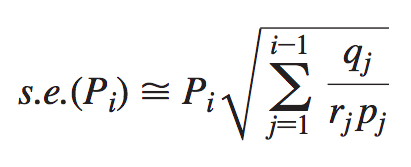
The hazard, also sometimes called the failure rate, is the rate of not surviving to the midpoint of an interval, given survival to the start of the interval.

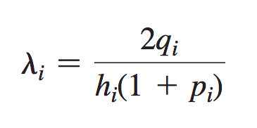
where h_i = the width of the ith interval.

The probability density is the probability of not surviving to the midpoint of an interval, given survival to the start of the interval:

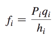
Note the distinction between the hazard function and the probability density function. The hazard function is the instantaneous rate of dropping out at a specific time among cases who survived to at least the beginning of that time interval. The probability density function is the probability of a given case dropping out at a specified time point.

What are plot of life tables?

Life table plots are simply the cumulative proportion surviving (Pi), plotted as a function of each time interval. 

How can you test for group differences in survival analysis?

Group differences in survival are tested through x² with degrees of freedom equal to the number of groups minus 1. Of the several tests that are available, the one demonstrated here is labeled Log-Rank in SAS LIFETEST and IBM SPSS KM. When there are only two groups, the overall test is equated as follows:

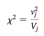
x² equals the squared value of the observed minus expected frequencies of number of survivors summed over all intervals for one of the groups (v²_j) under the null hypothesis of no group differences, divided by V_j, the variance of the group. The degree of freedom for this test is (number of groups -1). When there are only two groups, the value in the numerator is the same for both groups, but opposite in sign. The value in the denominator is also the same for both groups. Therefore, computations for either group produce the same x².

How is v_i calculated?

The value, v_i, of observed minus expected frequencies is calculated separately for each interval for one of the groups.

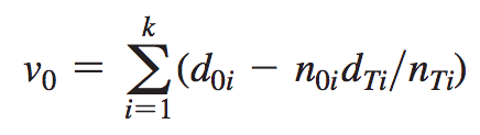
The difference between observed and expected frequencies for a group, v₀, is the summed differences over the intervals between the number of survivors in each interval, d0, minus the ratio of the number of cases at risk in the interval (n_0i) times the total number of survivors in that interval summed over all groups (d_Ti) divided by the total number of cases at risk in that interval summed over all groups (n_Ti).

How is V calculated?

The variance, V, for a group is calculated with the following formula:

The variance for the control group, V₀, is the sum over all intervals of the difference between the total number of survivors in an interval (n_Ti) times the number of survivors in the control group in the interval (n_0i) minus the squared number of survivors in the control group in the interval; this difference is multiplied by the product of the total number of survivors in the interval (d_Ti) times s_Ti(= n_Ti - d_Ti); all of this is divided by the squared total number of survivors in the interval (n_Ti) times the total number of survivors in the interval minus 1.

In jargon, the total number of cases that have survived to an interval (n_Ti) is called the risk set.

What different types of survival analyses are out there?

There are two major types of survival analyses:

• The first type is life tables, including proportions of survivors at various times and survivor functions, with tests of group differences. Life tables are estimated by either the actuarial or the product-limit (Kaplan–Meier) method.
• The other type is prediction of survival time from one or more covariates. Prediction of survival time from covariates most often involves the Cox proportional- hazards model (Cox regression).

How does the actuarial and product-limit life tables method work?

Both the actuarial method as well as the product-limit method can be used for calculating life tables. The two methods produce identical results when there is no censoring, and intervals contain no more than one time unit. 

The output is organized by time at which events occur rather than by time interval. For example, there are two lines of output for the two control cancer patients who dropped out during the second month and for the two cancer patients who dropped out in the tenth month. Both mean and median survival time are given, along with their standard errors and 95% confidence intervals. The survival-function chart differs slightly from that of the actuarial method by including information about cases that are censored. Group differences are tested through the Log Rank test, among others that can be requested, rather than the Wilcoxon test produced by IBM SPSS SURVIVAL.

How can group survival times be predicted from covariates?

Prediction of survival or failure time from covariates is similar to logistic regression but with provision for censored data. This method also differs in analyzing the time between events rather than predicting the occurrence of events. Cox proportional hazards (Cox regression) is the most popular method. Accelerated failure-time models are also available for the more sophisticated user.

As in other forms of regression, analysis of survival can be direct, sequential, or statistical. A treatment IV, if present, is analyzed the same as any other discrete covariate. When there are only two levels of treatment, the treated group is usually coded 1 and the control group 0. If there are more than two levels of treatment, dummy variable coding is used to represent group membership. Successful prediction on the basis of this IV indicates significant treatment effects.

What strategies can be used to conduct a survival analysis with covariates?

The three major analytic strategies in survival analysis with covariates are direct (standard), sequential (hierarchical), and statistical (stepwise or setwise). Differences among the strategies involve what happens to overlapping variability due to correlated covariates, including treatment groups, and who determines the order of entry of covariates into the equation.

• In the direct model all covariates enter the regression equation at one time and each is assessed as if it entered last. Therefore, each covariate is evaluated as to what it adds to prediction of survival time that is different from the prediction afforded by all the other covariates.
• In the sequential (sometimes called hierarchical) model, covariates enter the equation in an order specified by the researcher. Each covariate is assessed by what it adds to the equation at its own point of entry. Covariates are entered one at a time or in blocks. The analysis proceeds in steps, with information about the covariates in the equation given at each step. A typical strategy in survival analysis with an experimental IV is to enter all the nontreatment covariates at the first step, and then enter the covariate(s) representing the treatment variable at the second step. Output after the second step indicates the importance of the treatment variable to prediction of survival after statistical adjustment for the effects of other covariates.
• Statistical regression (sometimes generically called stepwise regression) is a controversial procedure in which order of entry of variables is based solely on statistical criteria. The meaning of the variables is not relevant. Decisions about which variables are included in the equation are based solely on statistics computed from the particular sample drawn; minor differences in these statistics can have a profound effect on the apparent importance of a covariate, including the one representing treatment groups. The procedure is typically used during early stages of research, when nontreatment covariates are being assessed for their relationship with survival. Covariates which contribute little to prediction are then dropped from subsequent research into the effects of treatment. As with logistic regression, data- driven strategies are especially dangerous when important decisions are based on results that may not generalize beyond the sample chosen. Cross- validation is crucial if statistical/stepwise techniques are used for any but the most preliminary investigations.

What does the Cox proportional-hazards model do?

The Cox proportional-hazards method models event rates as a log-linear function of predictors, called covariates. Regression coefficients give the relative effect of each covariate on the survivor function. Cox modeling is available through IBM SPSS COXREG and SAS PHREG.

Why is the choice of distribution important in accelerated failure-time models?

Accelerated failure-time models replace the general hazard function of the Cox model with a specific distribution. However, greater user sophistication is required to choose the distribution. Accelerated failure- time models are handled by SAS LIFEREG. IBM SPSS has no program for accelerated failure- time modeling. Choice of distributions in accelerated failure- time models has implications for hazard functions, so that modeling based on different distributions may lead to different interpretations. 

• Use of the exponential distribution assumes that the percentage for the hazard rate remains the same within a particular group of cases over time. 
• The Weibull distribution, on the other hand, permits the hazard rate for a particular group of cases to change over time. 
• The log-normal distribution looks like an inverted U-shaped distribution in which the hazard function rises to a peak and then declines as time goes by. This function is often associated with repeatable events.
• The log-logistic distribution also is an inverted U-shaped distribution when the scale parameter (σ) is less than 1, but behaves like the Weibull distribution when σ>1. It is a proportional-odds model, meaning that the change in log-odds is constant over time. A logistic distribution (without log-transform of time) may be specified in SAS LIFEREG.
• The gamma model (the one available in SAS LIFEREG is the generalized gamma model) is the most general model. Exponential, Weibull, and log-normal models are all special cases of it. Because of this relationship, differences between gamma and these other three models can be evaluated through likelihood ratio chi-square statistics. The gamma model can also have shapes that other models cannot, such as a U shape in which the hazard decreases over time to a minimum and then increases. Because there is no more general model than the gamma, there is no test of its adequacy as an underlying distribution. And because the model is so general, it will always provide at least as good a fit as any other model.

How can you make a choice for a specific model?

Choice of models is made on the basis of logic, graphical fit, or, in the case of nested models, goodness-of-fit tests. Allison has provided guidance for producing graphs of appropriate transformations to Kaplan– Meier estimates. A resulting linear plot indicates that the distribution providing the transformation is the appropriate one. Allison also illustrates procedures for applying goodness-of-fit statistics to statistically evaluate competing models. Accelerated failure- time analyses produce x² log- likelihood values, in which negative values closer to zero indicate better fits of data to models. Thus, twice the difference between nested models provides a likelihood- ratio χ² statistic. Of the nested models, gamma is the most general, followed by Weibull, then exponential, and finally lognormal. That is, log- normal is nested within exponential, which in turn is nested within Weibull, et cetera.

The most straightforward way to analyze survival data with covariates is Cox regression. It is more robust than accelerated failure-time methods and requires no choice among the distributions on the part of the researcher. However, the Cox model does have the assumption of proportionality of hazards over time.

What are some important issues when conducting a survival/failure analysis?

Issues in survival analysis include testing the assumption of proportionality of hazards, dealing with censored data, assessing effect size of models and individual covariates, choosing among the variety of statistical tests for differences among treatment groups and contributions of covariates, and interpreting hazard ratios.

What is meant with the proportionality of hazards assumption?

When Cox regression is used to analyze differences between levels of a discrete covariate such as treatment, it is assumed that the shapes of the survival functions are the same for all groups over time. That is, the time until failures begin to appear may be longer for one group than another, but once failures start, they proceed at the same rate for all groups. When the assumption is met, the lines for the survival functions for different groups are roughly parallel. Although inspection of the plots is helpful, a formal test of the assumption is also required. The assumption is similar to homogeneity of regression in ANCOVA, which requires that the relationship between the DV and the covariate(s) is the same for all levels of treatment.

The proportionality of hazards assumption is that the relationship between survival rate and time is the same for all levels of treatment (or any other covariate). In survival analysis, violation of proportionality signals interaction between time and levels of treatment (or any other covariate). To test the assumption, a time variable is constructed, and its interaction with levels of treatment (and other covariates) is tested.

How do censored data form an issue?

Censored cases are those for whom the time of the event being studied is unknown or only vaguely known.

• If failure has not occurred by the end of the study, the case is considered right-censored. Right-censoring is the most common form of censoring and occurs when the event being studied has not occurred by the time data collection ceases. Sometimes right-censoring is under the control of the researcher. Most methods of survival analysis do not distinguish among types of right-censoring, but cases that are lost from the study may pose problems because it is assumed that there are no systematic differences between them and the cases that remain.All of the programs reviewed here deal with right-censored data, but none distinguishes among the various types of right-censoring. Therefore, results are misleading if assumptions about censoring are violated.
• A case is left-censored if the event of interest occurred before an observed time, so that you know only that survival time is less than the total observation time. Left-censoring is unlikely to occur in an experiment, because random assignment to conditions is normally made only for intact cases. 
• With interval censoring, you know the interval within which the event occurred, but not the exact time within the interval. Interval censoring is likely to occur when events are monitored infrequently. 

A data set can contain a mix of cases with several forms of censoring.

How can the effect size be calculated in survival analysis?

Cox and Snell have provided a measure of effect size for logistic regression that is demonstrated for survival analysis by Allison. It is based on G2 , a likelihood-ratio chi-square statistic that can be calculated from SAS PHREG and LIFEREG and IBM SPSS COXREG. Models are fit both with and without covariates, and a difference G² is found by:

G² = [(-2 log-likelihood for smaller model) - (-2 log-likelihood for larger model)]  

Then, R² is found by:

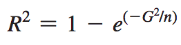
When applied to experiments, the R² of greatest interest is the association between survival and treatment, after adjustment for other covariates. Therefore, the smaller model is the one that includes covariates but not treatment, and the larger model is the one that includes covariates and treatment. Allison points out that this R² is not the proportion of variance in survival that is explained by the covariates, but merely represents relative association between survival and the covariates tested.

How can power be enhanced in survival analysis?

Power in survival analysis is, as usual, enhanced by larger sample sizes and covariates with stronger effects. Amount of censoring and patterns of entry of cases into the study also affect power. as does the relative size of treatment groups. Unequal sample sizes reduce power while equal sample sizes increase it.

What are the statistical criteria in survival/failure analysis?

Numerous statistical tests are available for evaluating group differences due to treatment effects from an actuarial life table or product-limit analysis.

• Several statistical tests are available for evaluating group differences. The tests differ primarily in how cases are weighted, with weighting based on the time that groups begin to diverge during the course of survival. For example, if the groups begin to diverge right away (untreated cases fail quickly but treated cases do not), statistics based on heavier weighting of cases that fail quickly show greater group differences than statistics for which all cases are weighted equally.
• Log-likelihood chi-square tests (G²) are used both to test the hypothesis that all regression coefficients for covariates are zero in a Cox proportional hazards model and to evaluate differences in models with and without a particular set of covariates. Statistics are also available to test regression coefficients separately for each covariate. These Wald tests are z-tests where the coefficient is divided by its standard error. When the test is applied to the treatment covariate, it is another test of the effect of treatment after adjustment for all other covariates.

How can we predict survival rate?

Statistics for predicting survival from covariates require calculating regression coefficients for each covariate where one or more of the covariates may represent treatment. The regression coefficients give the relative effect of each covariate on the survival function, but the size depends on the scale of the covariate. These coefficients may be used to develop a regression equation for risk as a DV.

What is the difference between the programs that can be used for survival analysis?

IBM SPSS and SAS have two or more programs that do different types of analysis. SAS has one program for survival functions and two for regression- type problems: one for proportional-hazards models and the other for various nonproportional-hazards models. IBM SPSS has three programs as well: one for proportional-hazards models and two for survival functions (one for actuarial and one for product-limit methods). SYSTAT has a single program for survival analysis.

What do canonical correlations entail? - Chapter 12

What are canonical correlations used for?

The goal of canonical correlation is to analyze the relationships between two sets of variables. It may be useful to think of one set of variables as IVs and the other set as DVs, or it may not. In any event, canonical correlation provides a statistical analysis for research in which each subject is measured on two sets of variables and the researcher wants to know if and how the two sets relate to each other.

The easiest way to understand canonical correlation is to think of multiple regression. In regression, there are several variables on one side of the equation and a single variable on the other side. The several variables are combined into a predicted value to produce, across all subjects, the highest correlation between the predicted value and the single variable. The combination of variables can be thought of as a dimension among the many variables that predicts the single variable. In canonical correlation, the same thing happens except that there are several variables on both sides of the equation. Sets of variables on each side are combined to produce, for each side, a predicted value that has the highest correlation with the predicted value on the other side. The combination of variables on each side can be thought of as a dimension that relates the variables on one side to the variables on the other. There is a complication, however. In multiple regression, there is only one combination of variables because there is only a single variable to predict on the other side of the equation. In canonical correlation, there are several variables on both sides and there may be several ways to recombine the variables on both sides to relate them to each other. 

What is the important jargon on canonical correlations?

Canonical correlation analysis is useful when the underlying dimensions representing the combinations of variables are unknown. Structural equations modelling may provide a more effective analysis when theory or prior research suggests the underlying dimensions. Thus, canonical analysis may be seen as an exploratory technique, with SEM as the parallel confirmatory technique. A good deal of the difficulty with canonical correlation is due to jargon. First, there are variables, then there are canonical variates, and, finally, there are pairs of canonical variates. Variables refer to the variables measured in research. Canonical variates are linear combinations of variables, one combination on the IV side and another combination on the DV side. These two combinations form a pair of canonical variates. However, there may be more than one significant pair of canonical variates. 

What kinds of research questions can be used for canonical analysis?

Although a large number of research questions are answered by canonical analysis in one of its specialized forms, relatively few intricate research questions are readily answered through direct application of computer programs currently available for canonical correlation. In part, this has to do with the programs themselves, and in part, it has to do with the kinds of questions researchers consider appropriate in a canonical correlation. In its present stage of development, canonical correlation is best considered a descriptive technique or a screening procedure rather than a hypothesis– testing procedure. 

• One type of research question relates to the number of canonical variate pairs. How many significant canonical variate pairs are there in the data set? Along how many dimensions are the variables in one set related to the variables in the other? 
• Another type relates to the interpretation of canonical variables. How are the dimensions that relate two sets of variables to be interpreted? What is the meaning in the combination of variables that compose one variate in conjunction with the combination composing the other in the same pair?
• The importance of canonical variates can also be assessed. There are several ways: The first is to ask how strongly the variate on one side of the equation relates to the variate on the other side of the equation; that is, how strong is the correlation between variates in a pair? A common measure is h2 = (1-Λ) as per MANOVA for the entire relationship among pairs of canonical variates. The second is to ask how strongly the variate on one side of the equation relates to the variables on its own side of the equation. The third is to ask how strongly the variate on one side of the equation relates to the variables on the other side of the equation.
• The last possibility is to define canonical variate scores. Had it been possible to measure directly the canonical variates from both sets of variables, what scores would subjects have received on them? Examination of canonical variate scores reveals deviant cases, the shape of the relationship between two canonical variates, and the shape of the relationships between canonical variates and the original variables. If canonical variates are interpretable, scores on them might be useful as IVs or DVs in other analyses.

What are the theoretical limitations of canonical analysis?

Canonical correlation has several important theoretical limitations that help explain its scarcity in the literature. Perhaps the most critical limitation is interpretability; procedures that maximize correlation do not necessarily maximize interpretation of pairs of canonical variates. Therefore, canonical solutions are often mathematically elegant but uninterpretable. And, although it is common practice in factor analysis and principal components analysis to rotate a solution to improve interpretation, rotation of canonical variates is not common practice or even available in some computer programs.

The algorithm used for canonical correlation maximizes the linear relationship between two sets of variables. If the relationship is nonlinear, the analysis misses some or most of it. If a nonlinear relationship between dimensions in a pair is suspected, use of canonical correlation may be inappropriate unless variables are transformed or combined to capture the nonlinear component. It is especially important in canonical analysis to emphasize that the use of terms IV and DV does not imply a causal relationship. 

In what way does the sensitivity of the solution form an important concern?

An important concern is the sensitivity of the solution in one set of variables to the variables included in the other set. In canonical analysis, the solution depends both on correlations among variables in each set and on correlations among variables between sets. Changing the variables in one set may markedly alter the composition of canonical variates in the other set. To some extent, this is expected given the goals of analysis; yet, the sensitivity of the procedure to apparently minor changes is a cause for concern.

What are the five practical issues of canonical analysis?

We distinguish five important practical issues of canonical analysis:

• The first concerns is the ratio of cases to IVs. The number of cases needed for analysis depends on the reliability of the variables. If reliability is very high, as, for instance, in political science where the variables are measures of the economic performance of countries, then a much lower ratio of cases to variables is acceptable. Power considerations are as important in canonical correlation as in other techniques, but software is less likely to be available to provide aid in determining sample sizes for expected effect sizes and desired power.
• The second concern relates to normality, linearity and homoscedasticity. Although there is no requirement that the variables be normally distributed when canonical correlation is used descriptively, the analysis is enhanced if they are. Normality, linearity, and homoscedasticity can be assessed through normal screening procedures or through the distributions of canonical variate scores produced by a preliminary canonical analysis. Inference regarding number of significant canonical variate pairs proceeds on the assumption of multivariate normality. Linearity is important to canonical analysis in at least two ways. The first is that the analysis is performed on correlation or variance– covariance matrices that reflect only linear relationships. The second is that the canonical correlation maximizes the linear relationship between a variate from one set of variables and a variate from the other set. Canonical analysis misses potential nonlinear components of relationships between canonical variate pairs. Finally, canonical analysis is best when relationships among pairs of variables are homoscedastic, that is, when the variance of one variable is about the same at all levels of the other variable.
• The third issue relates to missing data. Canonical correlation is quite sensitive to minor changes in a data set.
• The absence of outliers is also crucial. Cases that are unusual often have undue impact on canonical analysis. The search for univariate and multivariate outliers is conducted separately within each set of variables.
• Finally, multicollinearity and singularity are also important concerns. For both logical and computational reasons, it is important that the variables in each set and across sets are not too highly correlated with each other. 

What are the fundamental equations used in canonical analyses?

A data set that is appropriately analyzed through canonical correlation has several subjects, each measured on four or more variables. The variables form two sets with at least two variables in the smaller set. 

The first step in a canonical analysis is generation of a correlation matrix. In this case, however, the correlation matrix is subdivided into four parts: the correlations between the DVs (R_yy), the correlations between the IVs (R_xx), and the two matrices of correlations between DVs and IVs (R_xy and R_yx). The equations are all variants on the following equation:

R = R^-1_yyR_yxR^-1_xxR_xy

The canonical correlation matrix is a product of four correlation matrices, between DVs (inverted), between IVs (inverted), and between DVs and IVs.

How are eigenvalues and eigenvectors calculated?

Although computing eigenvalues and eigenvectors is best left to the computer, the relationship between a canonical correlation and an eigenvalue is simple, namely:

λ_i = r²_ci  

Each eigenvalue, λ_i, is equal to the squared canonical correlation, r²_ci, for the pair of canonical variates. Once the eigenvalue is calculated for each pair of canonical variates, canonical correlation is found by taking the square root of the eigenvalue. Canonical correlation, r_ci, is interpreted as an ordinary Pearson product- moment correlation coefficient. When r_ci is squared, it represents, as usual, overlapping variance between two variables, or, in this case, variates. Because r²_ci = λ_i, the eigenvalues themselves represent overlapping variance between pairs of canonical variates.

How can we test whether one set of r_cis significantly differs from zero?

Significance tests are available to test whether one or a set of r_cs differs from zero:

The significance of one or more canonical correlations is evaluated as a chi- square variable, where N is the number of cases, k_x is the number of variables in the IV set, ky is the number in the DV set, and the natural logarithm of lambda, see the following formula: This chi square has (k_x)(k_y) df.

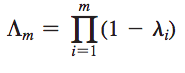
Lambda, Λ, is the product of differences between eigenvalues and unity, generated across m canonical correlations.

What do matrix equations look like?

Two sets of canonical coefficients (analogous to regression coefficients) are required for each canonical correlation, one set to combine the DVs and the other to combine the IVs. The canonical coefficients for the DVs are found as follows:

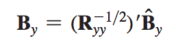
Canonical coefficients for the DVs are a product of (the transpose of the inverse of the square root of) the matrix of correlations between DVs and the normalized matrix of eigenvectors, Bn y, for the DVs. Once the canonical coefficients are computed, coefficients for the IVs are found using the following equation:

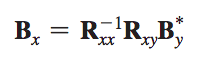
Coefficients for the IVs are a product of (the inverse of the square root of) the matrix of correlations between the IVs, the matrix of correlations between the IVs and DVs, and the matrix formed by the coefficients for the DVs - each divided by their corresponding canonical correlations.

The two matrices of canonical coefficients are used to estimate scores on canonical variates: X = Z_xB_x and Y = Z_yB_y. Scores on canonical variates are estimated as the product of the standardized scores on the original variates, Z_x and Z_y, and the canonical coefficients used to weight them, B_x and B_y.

Matrices of correlations between the variables and the canonical coefficients, called loading matrices, are used to interpret the canonical variates.

A_x = R_xxB_x and A_y = R_yyB_y  

Correlations between variables and canonical variates are found by multiplying the matrix of correlations between variables by the matrix of canonical coefficients.

How can you calculate the proportion of variance explained?

How much variance does each of the canonical variates extract from the variables on its own side of the equation? The proportion of variance extracted from the IVs by the canonical variates of the IVs is as follows:

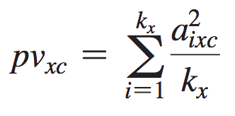
and

The proportion of variance extracted from a set of variables by a canonical variate of the set is the sum of the squared correlations divided by the number of variables in the set.

How can the redundancy be calculated?

Often, however, one is interested in knowing how much variance the canonical variates from the IVs extract from the DVs, and vice versa. In canonical analysis, this variance is called redundancy.

rd = (pv)(r²_c)

The redundancy in a canonical variate is the proportion of variance it extracts from its own set of variables times the squared canonical correlation for the pair.

What is the importance of canonical variates?

As in most statistical procedures, establishing significance is usually the first step in evaluating a solution. Conventional statistical procedures apply to significance tests for the number of canonical variate pairs. The number of statistically significant pairs of canonical variates is often larger than the number of interpretable pairs if N is at all sizable.

The only potential source of confusion is the meaning of the chain of significance tests. The first test is for all pairs taken together and is a test of independence between the two sets of variables. The second test is for all pairs of variates with the first and most important pair of canonical variates removed; the third is done with the first two pairs removed, and so forth.  

Once significance is established, amount of variance accounted for is of critical importance. Because there are two sets of variables, several assessments of variance are relevant. First, there is variance overlap between variates in a pair; second is a variance overlap between a variate and its own set of variables; and third is a variance overlap between a variate and the other set of variables.

• The first, and easiest, is the variance overlap between each significant set of canonical variate pairs. 
• The next consideration is the variance a canonical variate extracts from its own set of variables. A pair of canonical variates may extract very different amounts of variance from their respective sets of variables. 
• The last consideration is the variance a variate from one set extracts from the variables in the other set, called redundancy. A canonical variate from the IVs may be strongly correlated with the IVs, but weakly correlated with the DVs (and vice versa). Therefore, the redundancies for a pair of canonical variates are usually not equal. Because canonical variates are orthogonal, redundancies for a set of variables are also added across canonical variates to get a total for the DVs relative to the IVs, and vice versa.

How can you interpret canonical variates?

Canonical correlation creates linear combinations of variables, canonical variates, that represent mathematically viable combinations of variables. However, although mathematically viable, they are not necessarily interpretable. A major task for the researcher is to discern, if possible, the meaning of pairs of canonical variates.

Interpretation of significant pairs of canonical variates is based on the loading matrices, A_x and A_y. Each pair of canonical variates is interpreted as a pair, with a variate from one set of variables interpreted vis-à-vis the variate from the other set. A variate is interpreted by considering the pattern of variables highly correlated (loaded) with it. Because the loading matrices contain correlations, and because squared correlations measure overlapping variance, variables with correlations of .30 and above are usually interpreted as part of the variate, and variables with loadings below .30 are not. Deciding on a cutoff for interpreting loadings is, however, somewhat a matter of taste.

What different statistical programs can be used for canonical analysis?

One program is available in the SAS package for canonical analyses. IBM SPSS has two programs that may be used for canonical analysis. If available, the program of choice is SAS CANCORR and, with limitations, the IBM SPSS CANCORR macro.

What does canonical analysis look like in SAS CANCORR?

SAS CANCORR is a flexible program with abundant features and ease of interpretation. Along with the basics, you can specify easily interpretable labels for canonical variates and the program accepts several types of input matrices. Multivariate output is quite detailed, with several test criteria and voluminous redundancy analyses. Univariate output is minimal, however, and if plots are desired, case statistics such as canonical scores are written to a file to be analyzed by the SAS PLOT procedure.

If requested, the program does separate multiple regressions with each variable predicted from the other set. You can also do separate canonical correlation analyses for different groups.

What does canonical analysis look like in SPSS?

IBM SPSS has two programs for canonical analysis, both available only through syntax: IBM SPSS MANOVA and a CANCORR macro. A complete canonical analysis is available through SPSS MANOVA, which provides loadings, proportions of variance, redundancy, and much more. But problems arise with reading the results, because MANOVA is not designed specifically for canonical analysis and some of the labels are confusing. 

Canonical analysis is requested through MANOVA by calling one set of variables DVs and the other set covariates; no IVs are listed. Although IBM SPSS MANOVA provides a rather complete canonical analysis, it does not calculate canonical variate scores, nor does it offer multivariate plots.

What does canonical analysis look like in SYSTAT?

Currently, canonical analysis is most readily done through SETCOR SYSTAT System. The program provides all of the basics of canonical correlation and several others. There is a test of overall association between the two sets of variables, as well as tests of prediction of each DV from the set of IVs. The program also provides analyses in which one set is partialed from the other set––useful for statistical adjustment of irrelevant sources of variance (as per covariates in ANCOVA) as well as representation of curvilinear relationships and interactions. 

Canonical analysis may also be done through the multivariate general linear model GLM program in SYSTAT. But to get all the output, the analysis must be done twice, once with the first set of variables defined as the DVs, and a second time with the other set of variables defined as DVs. The advantages over SETCOR are that canonical variate scores may be saved in a data file, and that standardized canonical coefficients are provided.

What do principal components and factor analysis entail? - Chapter 13

What is the general purpose of PCA and FA?

Principal components analysis (PCA) and factor analysis (FA) are statistical techniques applied to a single set of variables when the researcher is interested in discovering which variables in the set form coherent subsets that are relatively independent of one another. Variables that are correlated with one another but largely independent of other subsets of variables are combined into factors. Factors are thought to reflect underlying processes that have created the correlations among variables. A major use of PCA and FA in psychology is in development of objective tests for measurement of personality and intelligence and the like.

The specific goals of PCA or FA are to summarize patterns of correlations among observed variables, to reduce a large number of observed variables to a smaller number of factors, to provide an operational definition (a regression equation) for an underlying process by using observed variables, or to test a theory about the nature of underlying processes. Some or all of these goals may be the focus of a particular research project. PCA and FA have considerable utility in reducing numerous variables down to a few factors. Mathematically, PCA and FA produce several linear combinations of observed variables, where each linear combination is a factor. The factors summarize the patterns of correlations in the observed correlation matrix and can be used, with varying degrees of success, to reproduce the observed correlation matrix. But since the number of factors is usually far fewer than the number of observed variables, there is considerable parsimony in using the factor analysis. Further, when scores on factors are estimated for each subject, they are often more reliable than scores on individual observed variables.

What are the steps in PCA and FA?

Steps in PCA or FA include selecting and measuring a set of variables, preparing the correlation matrix (to perform either PCA or FA), extracting a set of factors from the correlation matrix, determining the number of factors, (probably) rotating the factors to increase interpretability, and, finally, interpreting the results. Although there are relevant statistical considerations to most of these steps, an important test of the analysis is its interpretability.

How can a model be interpreted?

Interpretation and naming of factors depend on the meaning of the particular combination of observed variables that correlate highly with each factor. A factor is more easily interpreted when several observed variables correlate highly with it and those variables do not correlate with other factors. Once interpretability is adequate, the last, and very large, step is to verify the factor structure by establishing the construct validity of the factors. The researcher seeks to demonstrate that scores on the latent variables (factors) covary with scores on other variables, or that scores on latent variables change with experimental conditions as predicted by theory.

What are some problems in PCA and FA?

There are some problems when conducting PCA or FA.

• One of the problems with PCA and FA is that there are no readily available criteria against which to test the solution. There is no external criterion such as group membership against which to test the solution.
• A second problem with FA or PCA is that, after extraction, there is an infinite number of rotations available, all accounting for the same amount of variance in the original data, but with the factors defined slightly differently. The final choice among alternatives depends on the researcher’s assessment of its interpretability and scientific utility. 
• A third problem is that FA is frequently used in an attempt to 'save' poorly conceived research. If no other statistical procedure is applicable, at least data can usually be factor analyzed. Thus, in the minds of many, the various forms of FA are associated with sloppy research. The very power of PCA and FA to create apparent order from real chaos contributes to their somewhat tarnished reputations as scientific tools.

What are the two main types of factor analysis?

There are two major types of FA: exploratory and confirmatory.

• In exploratory FA, one seeks to describe and summarize data by grouping together variables that are correlated. The variables themselves may or may not have been chosen with potential underlying processes in mind. Exploratory FA is usually performed in the early stages of research, when it provides a tool for consolidating variables and for generating hypotheses about underlying processes.
• Confirmatory FA is a much more sophisticated technique used in the advanced stages of the research process to test a theory about latent processes. Variables are carefully and specifically chosen to reveal underlying processes. Currently, confirmatory FA is most often performed through structural equation modelling.

What is some important jargon in PCA and FA?

There are some important terms used in PCA and FA.

• The first terms involve correlation matrices. The correlation matrix produced by the observed variables is called the observed correlation matrix. The correlation matrix produced from factors, that is, correlation matrix implied by the factor solution, is called the reproduced correlation matrix. The difference between observed and reproduced correlation matrices is the residual correlation matrix. In a good FA, correlations in the residual matrix are small, indicating a close fit between the observed and reproduced matrices.
• A second set of terms refers to matrices produced and interpreted as part of the solution. Rotation of factors is a process by which the solution is made more interpretable without changing its underlying mathematical properties. There are two general classes of rotation: orthogonal and oblique. If rotation is orthogonal (so that all the factors are uncorrelated with each other), a loading matrix is produced. The loading matrix is a matrix of correlations between observed variables and factors. The sizes of the loadings reflect the extent of relationship between each observed variable and each factor. Orthogonal FA is interpreted from the loading matrix by looking at which observed variables correlate with each factor. If rotation is oblique (so that the factors themselves are correlated), several additional matrices are produced. The factor correlation matrix contains the correlations among the factors. The loading matrix from orthogonal rotation splits into two matrices for oblique rotation: a structure matrix of correlations between factors and variables and a pattern matrix of unique relationships (uncontaminated by overlap among factors) between each factor and each observed variable. Following oblique rotation, the meaning of factors is ascertained from the pattern matrix.
• Lastly, for both types of rotations, there is a factor-score coefficients matrix––a matrix of coefficients used in several regression-like equations to predict scores on factors from scores on observed variables for each individual.

What is the difference between PCA and FA?

FA produces factors, while PCA produces components. However, the processes are similar except in preparation of the observed correlation matrix for extraction and in the underlying theory. Mathematically, the difference between PCA and FA is in the variance that is analyzed. In PCA, all the variances in the observed variables are analyzed. In FA, only shared variance is analyzed; attempts are made to estimate and eliminate variance due to error and variance that is unique to each variable. The term factor is used here to refer to both components and factors unless the distinction is critical, in which case the appropriate term is used.

Theoretically, the difference between FA and PCA lies in the reason that variables are associated with a factor or component. Factors are thought to 'cause' variables - the underlying construct (the factor) is what produces scores on the variables. Thus, exploratory FA is associated with theory development and confirmatory FA is associated with theory testing.

• The question in exploratory FA is: What are the underlying processes that could have produced correlations among these variables?
• The question in confirmatory FA is: Are the correlations among variables consistent with a hypothesized factor structure? 

What type of research questions can be answered using PCA and FA?

The goal of research using PCA or FA is to reduce a large number of variables to a smaller number of factors, to concisely describe (and perhaps understand) the relationships among observed variables, or to test theory about underlying processes.

• One type of research question relates to the number of factors: How many reliable and interpretable factors are there in the data set? How many factors are needed to summarize the pattern of correlations in the correlation matrix? 
• A second type of questions relates to the nature of the factors: What is the meaning of the factors? How are the factors to be interpreted? Factors are interpreted by the variables that correlate with them.
• Then, research questions in PCA and FA can also relate to the importance of solutions and factors: How much variance in a data set is accounted for by the factors? Which factors account for the most variance? In a good factor analysis, a high percentage of the variance in the observed variables is accounted for by the first few factors. And, because factors are computed in descending order of magnitude, the first factor accounts for the most variance, with later factors accounting for less and less of the variance until they are no longer reliable
• Furthermore, FA can also be used for testing theories: How well does the obtained factor solution fit an expected factor solution? 
• Finally, scores on factors can be estimated: Had factors been measured directly, what scores would subjects have received on each of them?

What are some theoretical issues related to PCA and FA?

There are some theoretical considerations when using PCA or FA:

• Most applications of PCA or FA are exploratory in nature; FA is used primarily as a tool for reducing the number of variables or examining patterns of correlations among variables. Under these circumstances, both the theoretical and the practical limitations to FA are relaxed in favor of a frank exploration of the data. Decisions about number of factors and rotational scheme are based on pragmatic rather than theoretical criteria.
• The complexity of the variables is also considered. Complexity is indicated by the number of factors with which a variable correlates. A pure variable, which is preferred, is correlated with only one factor, whereas a complex variable is correlated with several. If variables differing in complexity are all included in an analysis, those with similar complexity levels may “catch” each other in factors that have little to do with underlying processes. Variables with similar complexity may correlate with each other because of their complexity and not because they relate to the same factor. Estimating (or avoiding) the complexity of variables is part of generating hypotheses about factors and selecting variables to measure them.
• In addition to this, it is also important that the sample chosen exhibits spread in scores with respect to the variables and the factors they measure. If all subjects achieve about the same score on some factor, correlations among the observed variables are low and the factor may not emerge in analysis. Selection of subjects expected to differ on the observed variables and underlying factors is an important design consideration.
• Finally, one should also be wary of pooling the results of several samples, or the same sample with measures repeated in time, for factor analytic purposes. First, samples that are known to be different with respect to some criterion may also have different factors. Examination of group differences is often quite revealing. Second, underlying factor structure may shift in time for the same subjects with learning or with experience in an experimental setting and these differences may also be quite revealing. Pooling results from diverse groups in FA may obscure differences rather than illuminate them.

What are some practical issues related to PCA and FA?

Because FA and PCA are exquisitely sensitive to the sizes of correlations, it is critical that honest correlations be employed. Sensitivity to outlying cases, problems created by missing data, and degradation of correlations between poorly distributed variables all plague FA and PCA.

• The first consideration relates to sample size. Correlation coefficients tend to be less reliable when estimated from small samples. Therefore, it is important that sample size be large enough that correlations are reliably estimated. The required sample size also depends on magnitude of population correlations and number of factors: if there are strong correlations and a few, distinct factors, a smaller sample size is adequate.
• Another consideration relates to missing data. If cases have missing data, either the missing values are estimated or the cases deleted

What are the assumptions of PCA and FA?

PCA and FA have several assumptions: normality, linearity, absence of outliers, and absence of multicollinearity and singularity.

• As long as PCA and FA are used descriptively as convenient ways to summarize the relationships in a large set of observed variables, assumptions regarding the distributions of variables are not in force. If variables are normally distributed, the solution is enhanced. To the extent that normality fails, the solution is degraded but may still be worthwhile. However, multivariate normality is assumed when statistical inference is used to determine the number of factors. Multivariate normality is the assumption that all variables, and all linear combinations of variables, are normally distributed. Although tests of multivariate normality are overly sensitive, normality among single variables is assessed by skewness and kurtosis.
• Multivariate normality also implies that relationships among pairs of variables are linear. The analysis is degraded when linearity fails, because correlation measures linear relationship and does not reflect nonlinear relationship. Linearity among pairs of variables is assessed through inspection of scatterplots.
• As in all multivariate techniques, cases may be outliers either on individual variables (univariate) or on combinations of variables (multivariate). Such cases have more influence on the factor solution than other cases.
• In PCA, multicollinearity is not a problem because there is no need to invert a matrix. For most forms of FA and for estimation of factor scores in any form of FA, singularity or extreme multicollinearity is a problem. For FA, if the determinant of R and eigenvalues associated with some factors approach 0, multicollinearity or singularity may be present. To investigate further, look at the SMCs for each variable where it serves as DV with all other variables as IVs. If any of the SMCs is one, singularity is present; if any of the SMCs is very large (near one), multicollinearity is present. Delete the variable with multicollinearity or singularity.

What does the factorability of R entail and how do you check for it?

A matrix that is factorable should include several sizable correlations. The expected size depends, to some extent, on N (larger sample sizes tend to produce smaller correlations), but if no correlation exceeds .30, use of FA is questionable because there is probably nothing to factor analyze. Inspect R for correlations in excess of .30, and, if none is found, reconsider use of FA.

High bivariate correlations, however, are not ironclad proof that the correlation matrix contains factors. It is possible that the correlations are between only two variables and do not reflect the underlying processes that are simultaneously affecting several variables. For this reason, it is helpful to examine matrices of partial correlations where pairwise correlations are adjusted for effects of all other variables. If there are factors present, then high bivariate correlations become very low partial correlations. IBM SPSS and SAS produce partial correlation matrices

How do you control for the absence of outliers among variables in PCA and FA?

After FA, in both exploratory and confirmatory FA, variables that are unrelated to others in the set are identified. These variables are usually not correlated with the first few factors although they often correlate with factors extracted later. These factors are usually unreliable, both because they account for very little variance and because factors that are defined by just one or two variables are not stable. Therefore, one never knows whether these factors are 'real'.

If the variance accounted for by a factor defined by only one or two variables is high enough, the factor is interpreted with great caution or is ignored, as pragmatic considerations dictate. In confirmatory FA done through FA rather than SEM programs, the factor represents either a promising lead for future work or (probably) error variance, but its interpretation awaits clarification by more research. A variable with a low squared multiple correlation with all other variables and low correlations with all important factors is an outlier among the variables. The variable is usually ignored in the current FA and either deleted or given friends in future research. 

What are the fundamental equations used for factor analysis?

The main variables that are used in PCA and FA are matrices of correlations (between variables, between factors, and between variables and factors), matrices of standard scores (on variables and on factors), matrices of regression weights (for producing scores on factors from scores on variables), and the pattern matrix of unique relationships between factors and variables after oblique rotation.

How does extraction work?

An important theorem from matrix algebra indicates that, under certain conditions, matrices can be diagonalized. Correlation and covariance matrices are among those that often can be diagonalized. When a matrix is diagonalized, it is transformed into a matrix with numbers in the positive diagonal and zeros everywhere else. In this application, the numbers in the positive diagonal represent variance from the correlation matrix that has been repackaged as follows:

L = V'RV

Diagonalization of R is accomplished by post- and pre- multiplying it by the matrix V and its transpose. The columns in V are called eigenvectors, and the values in the main diagonal of L are called eigenvalues. The first eigenvector corresponds to the first eigenvalue, and so forth.

Because there are four variables in the example, there are four eigenvalues with their corresponding eigenvectors. However, because the goal of FA is to summarize a pattern of correlations with as few factors as possible, and because each eigenvalue corresponds to a different potential factor, usually only factors with large eigenvalues are retained. In a good FA, these few factors almost duplicate the correlation matrix.

The matrix of eigenvectors pre- multiplied by its transpose produces the identity matrix with ones in the positive diagonal and zeros elsewhere. Therefore, pre- and post- multiplying the correlation matrix by eigenvectors does not change it so much as repackage it:

V'V = I

The important point is that because correlation matrices often meet requirements for diagonalizability, it is possible to use on them the matrix algebra of eigenvectors and eigenvalues with FA as the result. When a matrix is diagonalized, the information contained in it is repackaged. FA, the variance in the correlation matrix is condensed into eigenvalues. The factor with the largest eigenvalue has the most variance and so on, down to factors with small or negative eigenvalues that are usually omitted from solutions. Calculations for eigenvectors and eigenvalues are extremely laborious and not particularly enlightening.

R = VLV'

The correlation matrix can be considered a product of three matrices— the matrices of eigenvalues and corresponding eigenvectors.

How is the square root of the matrix of eigenvalues calculated?

After reorganization, the square root is taken of the matrix of eigenvalues:

or

If V√L is called A and √LV is A then R=AA'. The correlation matrix can also be considered a product of two matrices - each a combination of eigenvectors and the square root of eigenvalues. The factor loading matrix is a matrix of correlations between factors and variables.

What does orthogonal rotation entail?

Rotation is ordinarily used after extraction to maximize high correlations between factors and variables and minimize low ones. Numerous methods of rotation are available but the most commonly used, and the one illustrated here, is varimax. Varimax is a variance-maximizing procedure. The goal of varimax rotation is to maximize the variance of factor loadings by making high loadings higher and low ones lower for each factor. This goal is accomplished by means of a transformation matrix Λ.

A_unrotatedΛ = A_rotated

The unrotated factor loading matrix is multiplied by the transformation matrix to produce the rotated loading matrix. Compare the rotated and unrotated loading matrices. Notice that in the rotated matrix the low correlations are lower and the high ones are higher than in the unrotated loading matrix. Emphasizing differences in loadings facilitates interpretation of a factor by making unambiguous the variables that correlate with it. The numbers in the transformation matrix have a spatial interpretation.

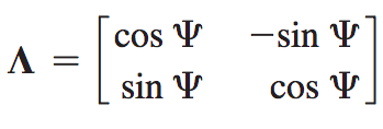
The transformation matrix is a matrix of sines and cosines of an angle ψ.

What do commonalities, variance and covariance entail?

Once the rotated loading matrix is available, other relationships are found. The communality for a variable is the variance accounted for by the factors. It is the squared multiple correlation of the variable as predicted from the factors. Communality is the sum of squared loadings (SSL) for a variable across factors. The proportion of variance in the set of variables accounted for by a factor is the SSL for the factor divided by the number of variables (if rotation is orthogonal). The proportion of variance in the solution accounted for by a factor - the proportion of covariance - is the SSL for the factor divided by the sum of communalities (or, equivalently, the sum of the SSLs). 

Notice that the reproduced correlation matrix differs slightly from the original correlation matrix. The difference between the original and reproduced correlation matrices is the residual correlation matrix:

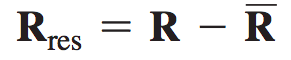
The residual correlation matrix is the difference between the observed correlation matrix and the reproduced correlation matrix.

How are factor scores calculated?

Scores on factors can be predicted for each case once the loading matrix is available. Regressionlike coefficients are computed for weighting variable scores to produce factor scores. 

B = R^-1A

Factor score coefficients for estimating factor scores from variable scores are a product of the inverse of the correlation matrix and the factor loading matrix. To estimate a subject’s score for the first factor, all of the subject’s scores on variables are standardized. In matrix form, F = ZB. Factor scores are a product of standardized scores on variables and factor score coefficients.

How can scores on variables be predicted from scores on factors?

Predicting scores on variables from scores on factors is also possible. The equation for doing so is:

Z = FA'

Predicted standardized scores on variables are a product of scores on factors weighted by factor loadings. A score on an observed variable is conceptualized as a properly weighted and summed combination of the scores on factors that underlie it. The researcher believes that each subject has the same latent factor structure, but different scores on the factors themselves. A particular subject’s score on an observed variable is produced as a weighted combination of that subject’s scores on the underlying factors.

What does oblique rotation entail?

All the relationships mentioned thus far are for orthogonal rotation. Most of the complexities of orthogonal rotation remain and several others are added when oblique (correlated) rotation is used. In oblique rotation, the loading matrix becomes the pattern matrix. Values in the pattern matrix, when squared, represent the unique contribution of each factor to the variance of each variable but do not include segments of variance that come from overlap between correlated factors. Once the factor scores are determined, correlations among factors can be obtained. Among the equations used for this purpose is:

One way to compute correlations among factors is from cross- products of standardized factor scores divided by the number of cases minus one. The factor correlation matrix is a standard part of computer output following oblique rotation. 

How can the structure matrix be calculated?

If oblique rotation is used, the structure matrix, C, is the correlations between variables and factors. These correlations assess the unique relationship between the variable and the factor (in the pattern matrix) plus the relationship between the variable and the overlapping variance among the factors. The equation for the structure matrix is:

C = AΦ

The structure matrix is a product of the pattern matrix and the factor correlation matrix. Most researchers interpret and report the pattern matrix rather than the structure matrix. However, if the researcher reports either the structure or the pattern matrix and also , then the interested reader can generate the other using the following formula. In oblique rotation, R, is produced as follows:

R = CA'

The reproduced correlation matrix is a product of the structure matrix and the transpose of the pattern matrix.

What are the major types of factor analysis?

Numerous procedures for factor extraction and rotation are available. However, only those procedures available in IBM SPSS and SAS packages are summarized here.

• The first group of techniques are factor extraction techniques. Among the extraction techniques available in the packages are principal components (PCA), principal factors, maximum likelihood factoring, image factoring, alpha factoring, and unweighted and generalized (weighted) least squares factoring. Of these, PCA and principal factors are the most commonly used. All the extraction techniques calculate a set of orthogonal components or factors that, in combination, reproduce R. Criteria used to establish the solution, such as maximizing variance or minimizing residual correlations, differ from technique to technique. But differences in solutions are small for a data set with a large sample, numerous variables, and similar communality estimates. 
• The second technique is rotation. The results of factor extraction, unaccompanied by rotation, are likely to be hard to interpret regardless of which method of extraction is used. After extraction, rotation is used to improve the interpretability and scientific utility of the solution. It is not used to improve the quality of the mathematical fit between the observed and reproduced correlation matrices because all orthogonally rotated solutions are mathematically equivalent to one another and to the solution before rotation. Varimax, quartimax, and equamax - three orthogonal techniques - are available. Varimax is easily the most commonly used of all the rotations available.

What are some important issues with PCA and FA?

Some of the issues raised in this section can be resolved through several different methods. Usually, different methods lead to the same conclusion; occasionally they do not. When they do not, results are judged by the interpretability and scientific utility of the solutions.

• FA differs from PCA in that communality values (numbers between 0 and 1) replace ones in the positive diagonal of R before factor extraction. Communality values are used instead of ones to remove the unique and error variance of each observed variable; only the variance a variable shares with the factors is used in the solution. But communality values are estimated, and there is some dispute regarding how that should be done.
• Because inclusion of more factors in a solution improves the fit between observed and reproduced correlation matrices, adequacy of extraction is tied to number of factors. The more factors extracted, the better the fit and the greater the percent of variance in the data “explained” by the factor solution. However, the more factors extracted, the less parsimonious the solution. To account for all the variance (PCA) or covariance (FA) in a data set, one would normally have to have as many factors as observed variables. It is clear, then, that a trade- off is required: One wants to retain enough factors for an adequate fit, but not so many that parsimony is lost.
• Furthermore, the decision between orthogonal and oblique rotation is made as soon as the number of reliable factors is apparent. In many factor analytic situations, oblique rotation seems more reasonable on the face of it than orthogonal rotation because it seems more likely that factors are correlated than that they are not. However, reporting the results of oblique rotation requires reporting the elements of the pattern matrix (A) and the factor correlation matrix (Φ) whereas reporting orthogonal rotation requires only the loading matrix (A). Thus, simplicity of reporting results favors orthogonal rotation. Further, if factor scores or factorlike scores are to be used as IVs or DVs in other analyses, or if a goal of analysis is comparison of factor structure in groups, then orthogonal rotation has distinct advantages.
• Then, the importance of a factor (or a set of factors) is evaluated by the proportion of variance or covariance accounted for by the factor after rotation. The proportion of variance attributable to individual factors differs before and after rotation because rotation tends to redistribute variance among factors somewhat. Ease of ascertaining proportions of variance for factors depends on whether rotation was orthogonal or oblique.
• Additionally, to interpret a factor, one tries to understand the underlying dimension that unifies the group of variables loading on it. In both orthogonal and oblique rotations, loadings are obtained from the loading matrix, A, but the meaning of the loadings is different for the two rotations.
• Finally, among the potentially more useful outcomes of PCA or FA are factor scores. Factor scores are estimates of the scores that subjects would have received on each of the factors had they been measured directly. Because there are normally fewer factors than observed variables, and because factor scores are nearly uncorrelated if factors are orthogonal, use of factor scores in other analyses may be very helpful. Multicollinear matrices can be reduced to orthogonal components using PCA, for instance.

What different statistical programs can be used for PCA and FA?

IBM SPSS, SAS, and SYSTAT each have a single program to handle both FA and PCA. The first two programs have numerous options for extraction and rotation and give the user considerable latitude in directing the progress of the analysis. 

How can SPSS be used for PCA and FA?

IBM SPSS FACTOR does a PCA or FA on a correlation matrix or a factor loading matrix, helpful to the researcher who is interested in higher- order factoring (extracting factors from previous FAs). Several extraction methods and a variety of orthogonal rotation methods are available. Oblique rotation is done using direct oblimin, one of the best methods currently available.

How can SAS FACTOR be used for PCA and FA?

SAS FACTOR is another highly flexible, full- featured program for FA and PCA. About the only weakness is in screening for outliers. SAS FACTOR accepts rotated loading matrices, as long as factor correlations are provided, and can analyze a partial correlation or covariance matrix (with specification of variables to partial out). There are several options for extraction, as well as orthogonal and oblique rotation. Maximum- likelihood estimation provides a x² test for number of factors. Standard errors may be requested for factor loadings with maximum- likelihood estimation and promax rotation. A target pattern matrix can be specified as a criterion for oblique rotation in confirmatory FA. Additional options include specification of proportion of variance to be accounted for in determining the number of factors to retain and the option to allow communalities to be greater than 1.0. The correlation matrix can be weighted to allow the generalized least squares method of extraction.

How can SYSTAT System be used for PCA and FA?

The current SYSTAT FACTOR program is less limited than earlier versions. Wilkinson (1990) advocated the use of PCA rather than FA because of the indeterminacy problem (Section 13.6.6). However, the program now does PFA (called IPA) as well as PCA and maximum likelihood (MLA) extraction. Four common methods of orthogonal rotation are provided, as well as provision for oblique rotation. SYSTAT FACTOR can accept correlation or covariance matrices as well as raw data.

The SYSTAT FACTOR program provides scree plots and plots of factor loadings and will optionally sort the loading matrix by size of loading to aid interpretation. Additional information is available by requesting that standardized component scores, their coefficients, and loadings be sent to a data file. Factor scores (from PFA or MLA) cannot be saved. Residual scores (actual minus predicted z-scores) also can be saved, as well as the sum of the squared residuals and a probability value for it.

What does structural equation modelling entail? - Chapter 14

What is the general purpose of structural equation modelling?

Structural equation modeling (SEM) is a collection of statistical techniques that allow a set of relationships between one or more IVs, either continuous or discrete, and one or more DVs, either continuous or discrete, to be examined. Both IVs and DVs can be either factors or measured variables. Structural equation modeling is also referred to as causal modeling, causal analysis, simultaneous equation modeling, analysis of covariance structures, path analysis, or confirmatory factor analysis (CFA). The latter two are actually special types of SEM. SEM allows questions to be answered that involve multiple regression analyses of factors. 

What are the important variables in structural equation modelling?

Several conventions are used in developing SEM diagrams. Measured variables, also called observed variables, indicators, or manifest variables, are represented by squares or rectangles. Factors have two or more indicators and are also called latent variables, constructs, or unobserved variables. Factors are represented by circles or ovals in path diagrams. Relationships between variables are indicated by lines; lack of a line connecting variables implies that no direct relationship has been hypothesized. Lines have either one or two arrows.

• A line with one arrow represents a hypothesized direct relationship between two variables, and the variable with the arrow pointing to it is the DV.
• A line with an arrow at both ends indicates an unanalyzed relationship, simply a covariance between the two variables with no implied direction of effect.

The part of the model that relates the measured variables to the factors is sometimes called the measurement model. 

What does specification entail?

The first step in a SEM analysis is specification of a model, so this is a confirmatory rather than an exploratory technique. The model is estimated, evaluated, and perhaps modified. The goal of the analysis might be to test a model, to test specific hypotheses about a model, to modify an existing model, or to test a set of related models.

What are the advantages and disadvantages of structural equation modelling?

There are a number of advantages to the use of SEM. When relationships among factors are examined, the relationships are free of measurement error because the error has been estimated and removed, leaving only common variance. Reliability of measurement can be accounted for explicitly within the analysis by estimating and removing the measurement error. Additionally, complex relationships can be examined. When the phenomena of interest are complex and multidimensional, SEM is the only analysis that allows complete and simultaneous tests of all the relationships.

Unfortunately, there is a small price to pay for the flexibility that SEM offers. With the ability to analyze complex relationships among combinations of discrete and continuous variables - both observed and latent - comes more complexity and more ambiguity. Indeed, there is quite a bit of jargon and many choices of analytic techniques. 

What kinds of research questions can be answered using structural equation modelling?

The data set is an empirical covariance matrix and the model produces an estimated population covariance matrix. The major question asked by SEM is, 'Does the model produce an estimated population covariance matrix that is consistent with the sample (observed) covariance matrix?' After the adequacy of the model is assessed, various other questions about specific aspects of the model are addressed.

• The adequacy of the model can be assessed. Parameters (path coefficients, variances, and covariances of IVs) are estimated to create an estimated population covariance matrix. If the model is good, the parameter estimates will produce an estimated matrix that is close to the sample covariance matrix. Closeness is evaluated primarily with the chi- square test statistic and fit indices.
• Then, SEM is also used for testing theories. Each theory (model) generates its own covariance matrix. Which theory produces an estimated population covariance matrix that is most consistent with the sample covariance matrix? Models representing competing theories in a specific research area are estimated, pitted against each other, and evaluated.
• The amount of variance in the variables accounted for by the factors can also be assessed.
• Furthermore, the reliability of the indicators can also be assessed. 
• Then, parameters estimates can be made as well. Estimates of parameters are fundamental to SEM analyses because they are used to generate the estimated population covariance matrix for the model. What is the path coefficient for a specific path?
• Another possible research question is: Does an IV directly affect a specific DV, or does the IV affect the DV through an intermediary, or mediating, variable? 
• Additionally, group differences can be assessed as well: Do two or more groups differ in their covariance matrices, regression coefficients, or means?
• Differences within and across people, across time can also be examined. This time interval can be years, days, or microseconds.
• Then, multilevel modelling is also a possibility. Independent variables collected at different nested levels of measurement can be used to predict dependent variables at the same level or other levels of measurement.
• Finally, latent class analysis (LCA) creates latent groups (classes) of people from measured variables and then often uses these groups in other SEM analyses. One common application of LCA is to estimate latent classes of people and then examine how the different groups change over time. 

What are some theoretical issues to structural equation modelling?

SEM is a confirmatory technique in contrast to exploratory factor analysis. It is used most often to test a theory - maybe just a personal theory - but a theory nonetheless. Indeed, one cannot do SEM without prior knowledge of, or hypotheses about, potential relationships among variables. This is perhaps the largest difference between SEM and other techniques in this book and one of its greatest strengths. Planning, driven by theory, is essential to any SEM analysis.Although SEM is a confirmatory technique, there are ways to test a variety of different models after a model has been estimated. However, if numerous modifications of a model are tested in hopes of finding the best- fitting model, the researcher has moved to exploratory data analysis and appropriate steps need to be taken to protect against inflated Type I error levels. Searching for the best model is appropriate, provided significance levels are viewed cautiously and cross- validation with another sample is performed whenever possible.

SEM has developed a bad reputation in some circles, in part because of the use of SEM for exploratory work without the necessary controls. It may also be due, in part, to the use of the term causal modeling to refer to SEM. There is nothing causal, in the sense of inferring causality, about the use of SEM. Attributing causality is a design issue, not a statistical issue.

Why should we consider sample size in SEM?

Covariances, like correlations, are less stable when estimated from small samples. SEM is based on covariances. Parameter estimates and chi-square tests of fit are also very sensitive to sample size. SEM, then, like factor analysis, is a large sample technique. Models with strong expected parameter estimates and reliable variables may require fewer participants. Although SEM is a large sample technique, new test statistics have been developed that allow for estimation of models with as few as 60 participants

Why should we consider missing data in SEM?

Problems are associated with either deleting or estimating missing data. An advantage of structural modeling is that the missing data mechanism can be included in the model. Some of the software packages now include procedures for estimating missing data, including the EM algorithm.

What are the assumptions of structural equation modelling?

Structural equation modelling has several assumption:

• Most of the estimation techniques used in SEM assume multivariate normality. To determine the extent and shape of non-normally distributed data, screen the measured variables for outliers (both univariate and multivariate), and the skewness and kurtosis of the measured variables.
• SEM techniques examine only linear relationships among variables. Linearity among latent variables is difficult to assess; however, linear relationships among pairs of measured variables can be assessed through inspection of scatterplots. If nonlinear relationships among measured variables are hypothesized, these relationships are included by raising the measured variables to powers, as in multiple regression.
• As with the other techniques discussed in the book, matrices need to be inverted in SEM. Therefore, if variables are perfect linear combinations of one another or are extremely highly correlated, the necessary matrices cannot be inverted. If possible, inspect the determinant of the covariance matrix. An extremely small determinant may indicate a problem with multicollinearity or singularity. 
• After model estimation, the residuals should be small and centered around zero. The frequency distribution of the residual covariances should be symmetrical. Residuals in the context of SEM are residual covariances not residual scores as discussed in other chapters. SEM programs provide diagnostics of residuals. Nonsymmetrically distributed residuals in the frequency distribution may signal a poor- fitting model; the model is estimating some of the covariances well and others poorly. 

What are the fundamental equations used for structural equation modelling?

The idea behind SEM is that the hypothesized model has a set of underlying parameters which correspond to the regression coefficients, and the variances and covariances of the independent variables in the model. These parameters are estimated from the sample data to be a 'best guess' about population values. The estimated parameters are then combined by means of covariance algebra to produce an estimated population covariance matrix. This estimated population covariance matrix is compared with the sample covariance matrix and, ideally, the difference is very small and not statistically significant.

What does covariance algebra entail?

Covariance algebra is a helpful tool in calculating variances and covariances in SEM models; however, matrix methods are generally employed because covariance algebra becomes extremely tedious as models become increasingly complex. Covariance algebra is useful to demonstrate how parameter estimates are combined to produce an estimated population covariance matrix for a small example. The three basic rules in covariance algebra appear below where c is a constant and Xi is a random variable:

• COV (c, X₁) = 0 
• COV (cX₁, X_x) = cCOV (X₁, X₂) 
• COV (X₁ + X₂, X₃) = COV (X₁, X3) + COV (X₂, X₃)

By the first rule, the covariance between a variable and a constant is zero. By the second rule, the covariance between two variables where one is multiplied by a constant is the same as the constant multiplied by the covariance between the two variables. By the third rule, the covariance between the sum (or difference) of two variables and a third variable is the sum of the covariance of the first variable and the third and the covariance of the second variable and the third.

How do you specify the model?

To specify the model, a separate equation is written for each DV. For motivation, Y_1:

Y₁ = γ₁₁X₁ + ε₁ 

To calculate the covariance between X1 (treatment group) and Y1 (dependent variable), the first step is substituting in the equation for Y1:

COV (X₁, Y₁) = COV (X₁, γ₁₁X₁ + ε₁)

The second step is distributing the first term, in this case X1:

COV (X₁, Y₁) = COV (X₁γ₁₁X₁) + COV (X₁ε₁)

The last term in this equation, COV (X₁ε₁), is equal to zero by assumption because it is assumed that there are no covariances between errors and other variables. Now:

COV (X₁, Y₁) = γ₁₁COV (X₁X₁)

by rule 2, and because the covariance of a variable with itself is just a variance,

COV (X₁Y₁) = γ₁₁σ_X1X1 

The estimated population covariance between X₁ and Y₁ is equal to the path coefficient times the variance of X₁. This is the population covariance between X₁ and Y₁ as estimated from the model. If the model is good, the product of γ₁₁σ_X1X1 produces a covariance that is very close to the sample covariance.

Following the same procedures, the covariance between Y1 and Y2 is:

COV (Y₁, Y₂) = COV (γ₁₁X₁ + ε₁, β₂₁Y₁ + γ₂₁X₁ + ε₂)
= COV (γ₁₁X₁β₂₁Y₁) + COV (γ₁₁X₁γ₂₁X₁) + COV (γ₁₁X₁ε₂) + COV (ε₁β₂₁Y1) + COV (ε₁γ₂₁X₁) + COV (ε₁ε₂) = COV (γ₁₁β₂₁σ_X1Y1) + COV (γ₁₁γ₂₁σ_X1Y1)

because, as can be seen in the diagram, the error terms e1 and e2 do not correlate with any other variables.

What does the Bentler-Weeks method entail?

One method of model specification is the Bentler-Weeks method. In this method, every variable in the model, latent or measured, is either an IV or a DV. The parameters to be estimated are the (1) regression coefficients, and (2) the variances and the covariances of the independent variables in the model. Residual variables (errors) of measured variables are labeled E and errors of latent variables (called disturbances) are labeled D. It may seem odd that a residual variable is considered an IV but remember the familiar regression equation:

Y = Xβ + ε

where Y is the DV and X and ε are both IVs. In fact, the Bentler-Weeks model is a regression model, expressed in matrix algebra:

η = Bη + γξ  

where, if q is the number of DVs and r is the number of IVs, then η (eta) is a q*1 vector of DVs, β (beta) is a q*q matrix of regression coefficients between DVs, γ (gamma) is a q *r matrix of regression coefficients between DVs and IVs, and ξ (xi) is an r*1 vector of IVs.

In the Bentler-Weeks model, only independent variables have covariances and these covariances are in Φ (phi), an r*r matrix. Therefore, the parameter matrices of the model are B, γ, and Φ. Unknown parameters in these matrices need to be estimated. The vectors of dependent variables, η, and independent variables, ξ, are not estimated.

How do you calculate the estimated population covariance matrix?

To calculate the estimated population covariance matrix implied by the parameter estimates, selection matrices are first used to pull the measured variables out of the full parameter matrices. The selection matrix is simply labeled G and has elements that are either 1s or 0s. The resulting vector is labeled Y:

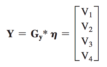
where Y is our name for the those measured variables that are dependent.

The independent measured variables are selected in a similar manner,

X = G_X * ξ = V5

where X is our name for the independent measured variables. Computation of the estimated population covariance matrix proceeds by rewriting the basic structural modeling as:

η = (I - B)^-1γξ 

where I is simply an identity matrix the same size as B. This equation expresses the DVs as a linear combination of the IVs. At this point, the estimated population covariance matrix for the DVs, Σyy, is estimated using:

The estimated population covariance matrix between IVs and DVs is obtained similarly by:

Finally, the estimated population covariance matrix between IVs is estimated:

What does model evaluation entail?

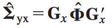
A χ² statistic is computed based upon the function minimum when the solution has converged. The χ² is evaluated with degrees of freedom equal to the difference between the total number of degrees of freedom and the number of parameters estimated. The degrees of freedom in SEM are equal to the amount of unique information in the sample variance/covariance matrix (variances and covariances) minus the number of parameters in the model to be estimated (regression coefficients and variances and covariances of independent variables). In a model with a few variables, it is easy to count the number of variances and covariances; however, in larger models, the number of data points is calculated as,

number of data points = (p(p + 1)) / 2

where p equals the number of measured variables.

Next, researchers usually examine the statistically significant relationships within the model. If the unstandardized coefficients in the three parameter matrices are divided by their respective standard errors, a z-score is obtained for each parameter that is evaluated in the usual manner:

z = parameter estimate / std error for estimate 

Freeing a parameter means estimating the parameter. 

What are some problems in the process of model identification?

In SEM, a model is specified, parameters for the model are estimated using sample data, and the parameters are used to produce the estimated population covariance matrix. But only models that are identified can be estimated. A model is said to be identified if there is a unique numerical solution for each of the parameters in the model. For example, say both that the variance of Y = 10 and that the variance of Y = α + β. Any two values can be substituted for a and b as long as they sum to 10. There is no unique numerical solution for either α or β, that is, there are an infinite number of combinations of two numbers that would sum to 10. Therefore, this single equation model is not identified. However, if we fix a to zero, then there is a unique solution for b, 10, and the equation is identified. It is possible to use covariance algebra to calculate equations and assess identification in very simple models; however, in large models, this procedure quickly becomes unwieldy.

• The first step is to count the numbers of data points and the number of parameters that are to be estimated. The data in SEM are the variances and covariances in the sample covariance matrix.
• The second step in determining model identifiability is to examine the measurement portion of the model. The measurement part of the model deals with the relationship between the measured indicators and the factors. It is necessary both to establish the scale of each factor and to assess the identifiability of this portion of the model.
• The third step in establishing model identifiability is to examine the structural portion of the model, looking only at the relationships among the latent variables (factors). Ignore the measured variables for a moment, and consider only the structural portion of the model that deals with the regression coefficients relating latent variables to one another. If none of the latent DVs predicts each other (the beta matrix is all zeros), the structural part of the model may be identified.

What are some estimation techniques?

After a model is specified, population parameters are estimated with the goal of minimizing the difference between the observed and estimated population covariance matrices. To accomplish this goal, a function, Q, is minimized where

Q = (s - σ(Θ))'W(s - σ(Θ))

where s is the vector of data (the observed sample covariance matrix stacked into a vector); σ is the vector of the estimated population covariance matrix (again, stacked into a vector); and Θ indicates that σ is derived from the parameters (the regression coefficients, variances, and covariances) of the model. W is the matrix that weights the squared differences between the sample and estimated population covariance matrix.

The trick is to select W to minimize the squared differences between observed and estimated population covariance matrices.

How do you assess the fit of the model?

After the model has been specified and then estimated, the major question is, “Is it a good model?” One component of a “good” model is the fit between the sample covariance matrix and the estimated population covariance matrix. Like multiway frequency analysis and logistic regression, a good fit is sometimes indicated by a nonsignificant χ². Unfortunately, assessment of fit is not always as straightforward as assessment of χ². With large samples, trivial differences between sample and estimated population covariance matrices are often significant because the minimum of the function is multiplied by N – 1. With small samples, the computed χ² may not be distributed as χ², leading to inaccurate probability levels. Finally, when assumptions underlying the χ²test statistic are violated, the probability levels are inaccurate.

One method of conceptualizing goodness of fit is by thinking of a series of models all nested within one another. Nested models are like the hierarchical models in log- linear modeling discussed in Chapter 16. Nested models are models that are subsets of one another. At one end of the continuum is the independence model: the model that corresponds to completely unrelated variables. This model would have degrees of freedom equal to the number of data points minus the variances that are estimated. At the other end of the continuum is the saturated (full or perfect) model with zero degrees of freedom. Fit indices that employ a comparative fit approach place the estimated model somewhere along this continuum.

The Bentler-Bonett normed fit index (NFI) evaluates the estimated model by comparing the χ² value of the model to the χ² value of the independence model.

NFI =  χ²_indep -  χ²_model /  χ²_indep 

This yields a descriptive fit index that lies in the 0-1 range. High values (greater than .95) are indicative of a good-fitting model.

What are the reasons for modifying a model?

There are at least two reasons for modifying a SEM model: to improve fit (especially in exploratory work) and to test hypotheses (in theoretical work). The three basic methods of model modification are chi- square difference tests, Lagrange multiplier tests (LM), and Wald tests. All are asymptotically equivalent under the null hypothesis (act the same as the sample size approaches infinity) but approach model modification differently.

• If models are nested (one model is a subset of another), the  χ² value for the larger model is subtracted from the  χ² value for the smaller nested model and the difference, also a  χ², is evaluated with degrees of freedom equal to the difference between the degrees of freedom in the two models. When the data are normally distributed, the chi- squares can simply be subtracted. However, when the data are nonnormal and the Satorra–Bentler scaled chi-square is employed, an adjustment is required so that the Satorra–Bentler chi-square is distributed as a chi-square.
• The LM test also compares nested models but requires estimation of only one model. The LM test asks if the model is improved if one or more of the parameters in the model that are currently fixed are estimated. Or, equivalently, what parameters should be added to the model to improve the fit? This method of model modification is analogous to forward stepwise regression.
• While the LM test asks which parameters, if any, should be added to a model, the Wald test asks which, if any, could be deleted. Are there any parameters that are currently being estimated that could, instead, be fixed to zero? Or, equivalently, which parameters are not necessary in the model? The Wald test is analogous to backward deletion of variables in stepwise regression where one seeks a nonsignificant change in the equation when variables are left out.

How do you assess reliability?

Reliability is defined in the classic sense as the proportion of true variance relative to total variance (true plus error variance). Both the reliability and the proportion of variance of a measured variable are assessed through squared multiple correlation (SMC) where the measured variable is the DV and the factor is the IV. Each SMC is interpreted as the reliability of the measured variable in the analysis and as the proportion of variance in the variable that is accounted for by the factor, conceptually the same as a communality estimate in factor analysis. To calculate a SMC:

SMC_{var i} = λ²_i / (λ²_i + Θ_ii)

The factor loading for variable i is squared and divided by that value plus the residual variance associated with the variable i.

This equation is applicable only for when there are no complex factor loadings or correlated errors. The proportion of variance in the variables accounted for by the factor is assessed as:

R_j² = 1 - D_j²

The disturbance (residual) for the DV factor j is squared and subtracted from 1.

How do you conduct SEM with discrete and ordinal data?

SEM assumes that measured variables are continuous and measured on an interval scale. Often, however, a researcher desires to include discrete and/or ordinally measured, categorical variables in an analysis. Because the data points in SEM are variances and covariances, the trick is to produce reasonable values for these types of variables for analysis.

Can you also estimate and compare models from two or more samples using SEM?

Although each of the models estimated in this chapter uses data from a single sample, it is also possible to estimate and compare models that come from two or more samples, called multiple group models. The general null hypothesis tested in multiple group models is that the data from each group are from the same population. For example, if data from a sample of men and a sample of women are drawn for the small- sample example, the general null hypothesis tested is that the two groups are drawn from the same population. The analysis begins by developing good- fitting models in separate runs for each group. The models are then tested in one run with none of the parameters across models constrained to be equal. This unconstrained multiple group model serves as the baseline against which to judge more restricted models.

Following baseline model estimation, progressively more stringent constraints are specified by constraining various parameters across all groups. When parameters are constrained, they are forced to be equal to one another. After each set of constraints is added, a chi-square difference test is performed for each group between the less restrictive and more restrictive model. The goal is to not degrade the models by constraining parameters across the groups; therefore, you want a nonsignificant χ². If a significant difference in  χ² is found between the models at any stage, the LM test is examined to locate the specific parameters that are different in the groups and these parameters are estimated separately in each group; that is, the specific across-group parameter constraints are released.

What statistical programs can be used for structural equation modelling?

The four SEM programs discussed - EQS, LISREL, SAS CALIS, and AMOS - are full-service, multioption programs.

• EQS is the most user-friendly of the programs. The equation method of specifying the model is clear and easy to use and the output is well organized. 
• LISREL offers residual diagnostics, several estimation methods, and many fit indices. LISREL includes two types of partially standardized solutions.
• AMOS allows models to be specified through diagrams or equations. Different options are available for the equation method. AMOS makes clever use of colors in the equation specification method. 
• SAS CALIS offers a choice of model specification methods:lineqs (Bentler–Weeks), ram, and cosan (a form of matrix specification). Diagnostics are available for evaluation of assumptions; for instance, evaluations of multivariate outliers and multivariate normality can be done within CALIS. If data are nonnormal, but with homogenous kurtosis, the chi- square test statistics can be adjusted within the program. Several different estimation techniques are available and lots of information about the estimation process is given. Categorical data are not treated in CALIS, nor can multiple group models be tested.

What does multilevel linear modelling entail? - Chapter 15

What is the general purpose of multilevel linear modelling?

Multilevel (hierarchical) linear modeling (MLM) is used for research designs, where the data for participants are organized at more than one level. Different variables may be available for each level of analysis. MLM provides an alternative analysis to several different designs discussed elsewhere in this volume. Although the lowest level of data in MLM is usually an individual, it may instead be repeated measurements of individuals. Another useful application of MLM is as an alternative to ANCOVA, where DV scores are adjusted for covariates (individual differences) prior to testing treatment differences.

An advantage of MLM over alternative analyses is that independence of errors is not required. In fact, independence is often violated at each level of analysis. In addition, there may be interactions across levels of the hierarchy. Analyzing data organized into hierarchies as if they are all on the same level leads to both interpretational and statistical errors. A less common but equally misleading approach is to interpret individual-level analyses at the group level, leading to the atomistic fallacy. A multilevel model, on the other hand, permits prediction of individual scores adjusted for group differences as well as prediction of group scores adjusted for individual differences within groups. Statistically, if individual scores are used without taking into account the hierarchical structure, the Type I error rate is inflated because analyses are based on too many degrees of freedom that are not truly independent.

Why are multilevel models often called random coefficient regression models?

Multilevel models often are called random coefficient regression models because the regression coefficients (the intercepts and predictor slopes) may vary across groups (higher-level units), which are considered to be randomly sampled from a population of groups. In garden-variety (OLS) regression, it is the individual participants who are considered to be a random sample from some population; in multilevel modelling, the groups also are considered to be a random sample.

One advantage of the multilevel modelling approach over other ways of handling hierarchical data is the opportunity to include predictors at every level of analysis.

What kinds of research questions can be answered using multilevel modelling?

The primary questions in MLM are like the questions in multiple regression: degree of relationship among the DV and various IVs; importance of IVs; adding and changing IVs; contingencies among IVs; parameter estimates; and predicting DV scores for members of a new sample. However, additional questions can be answered when the hierarchical structure of the data is taken into account and random intercepts and slopes are permitted. 

• Group differences in means can be assessed. This question is answered as part of the first step in routine hierarchical analyses. Is there a significant difference in intercepts (means) for the various groups?
• Then, group differences in slopes can also be assessed. This question may also be answered as part of routine hierarchical analyses. Is there a significant difference in slopes for the various groups?
• In addition, cross-level interactions can be assessed as well. Does a variable at one level interact with a variable at another level in its effect on the DV?
• MLM also provides a useful strategy for meta- analyses in which the goal is to compare many studies from the literature that address the same outcome. A common outcome measure is derived for the various studies, often a standardized effect size for the outcome measure.
• The relative strength of predictors at various levels can also be assessed. What is the relative size of the effect for individual-level variables versus group-level variables? Or, are interventions better aimed at the individual level or the group level? 
• Individual and group structures can also be analysed. Is the factor structure of a model the same at the individual and group level?
• Effect size can also be analysed. How much of the total variance in behavior is associated with predictors? 
• Furthermore, path analysis at individual and group levels can also be conducted. What is the path model for prediction of the DV from level-1, level-2, and level-3 variables?
• Then, longitudinal data can also be analysed. What is the pattern of change over time on a measure?
• Multilevel logistic regression is another application. What is the probability of a binary outcome when individuals are nested within several levels of a hierarchy? 
• Finally, multiple response analysis is another application of multilevel modelling. What are the effects of variables at different levels on multiple DVs at the individual level? 

What are some theoretical limitations to multilevel linear modelling?

Correlated predictors are even more problematic in MLM than in simple linear regression. In MLM, equations at multiple levels are solved and correlations among predictors at all levels are taken into account simultaneously. Because effects of correlated predictors are all adjusted for each other, it becomes increasingly likely that none of their regression coefficients will be statistically significant. The best advice, then, is to choose a very small number of relatively uncorrelated predictors. A strong theoretical framework helps limit the number of predictors and facilitates decisions about how to treat them.

If interactions are formed, predictors in the interactions are bound to be correlated with their main effects. The problem of multicollinearity between interactions and their main effects can be solved by centering. Modeling high-level predictors at their own level is not always the best way to deal with them. If there are only a few of them, they are often best entered at the next lower level as categorical predictors.

Why should sample size be considered in multilevel linear modelling?

The price of large, complex models is instability and a requirement for a substantial sample size at each level. Even small models, with only a few predictors, grow rapidly as equations are added at higher levels of analysis. Therefore, large samples are necessary even if there are only a few predictors. As a maximum likelihood technique, a sample size of at least 60 is required if only 5 or fewer parameters are estimated. Parameters to be estimated include intercepts and slopes as well as effects of interest at each level. In practice, convergence often is difficult even with larger sample sizes.

As in most analyses, increasing sample sizes increases power, while smaller effect sizes and larger standard errors decrease power.

What are the assumptions of multilevel linear modelling?

Multilevel linear modelling has several assumptions that need to be met.

• MLM is designed to deal with the violation of the assumption of independence of errors expected when individuals within groups share experiences that may affect their responses. The problem is similar to that of heterogeneity of covariance (sphericity), in that events that are close in time are more alike than those farther apart. In MLM, it usually is the individuals within groups who are closer to each other in space and experiences than to individuals in other groups. Indeed, when the lowest level of the hierarchy is repeated measures over time, multilevel modeling provides an alternative to the assumption of heterogeneity of covariance (sphericity) required in repeated- measures ANOVA.
• Collinearity among predictors is especially worrisome when cross- level interactions are formed, as is common in MLM, because these interactions are likely to be highly correlated with their component main effects. At the least, the problem often leads to a failure of significance for the main effect(s). At worst, multicollinearity can cause a failure of the model to converge on a solution. The solution is to center predictors.

What are the fundamental equations of multilevel linear modelling?

Small data sets are difficult to analyze through MLM. The maximum likelihood procedure fails to converge with multiple equations unless samples are large enough to support those equations. Nor is it convenient to apply MLM to a matrix (or a series of matrices). MLM is often conducted in a sequence of steps. Therefore, the equations and computer analyses are divided into three models of increasing complexity.

1. The first is an intercepts-only (null) model, in which there are no predictors and the test is for mean differences between X on the DV. 
2. The second is a model in which the first-level predictor is added to the intercepts-only model.
3. The third is a model in which the second-level predictor is added to the model with the first-level predictor.

The MLM is expressed as a set of regression equations. In the level-1 equation for the interceptsonly model (a model without predictors), the response (DV score) for an individual is predicted by an intercept that varies across groups. The intercepts-only model is of singular importance in MLM because it provides information about the intraclass correlation, a value helpful in determining whether a multilevel model is required or not.

What does the level-1 equation look like?

In the level-1 equation for the interceptsonly model (a model without predictors), the response (DV score) for an individual is predicted by an intercept that varies across groups.

Y_ij = β_0j + e_ij

An individual score on the DV, Y_ij, is the sum of an intercept (mean), β_0j, that can vary over the j groups and individual error, e_ij (the deviation of an individual from her or his group mean). The terms Y and e that in ordinary regression have a single subscript i, indicating case, now have two subscripts, ij, indicating case and group. The intercept, β₀ now also has a subscript, j, indicating that the coefficient varies over groups. That is, each group could have a separate equation.

β_0j is not likely to have a single value because its value depends on the group. Instead, a parameter estimate (τ₀₀) and standard error are developed for the variance of a random effect. The parameter estimate reflects the degree of variance for a random effect; large parameter estimates reflect effects that are highly variable. These parameter estimates and their significance tests are shown in computer runs to follow. The z test of the random component, τ₀₀ divided by its standard error, evaluates whether the groups vary more than that would be expected by chance.

What does the level-2 equation look like?

The second-level analysis (based on groups as research units) for the intercepts-only model uses the level-1 intercept (group mean) as the DV. To predict the intercept for group j:

β_oj = γ₀₀ + u_oj 

An intercept for a run, β_oj, is predicted from the average intercept over groups when there are no predictors, γ₀₀, and group error, u_oj (deviation from average intercept for group j). A separate equation could be written for each group.

Y_ij = γ₀₀ + u_oj + eij 

The average intercept (mean) is γ₀₀ (a fixed component). The two random components are u_oj (the deviation in intercept for cases in group j) and e_j (the deviation for case i from its group j).  

What does the model with predictors at first and second levels look like?

The full model adds a second-level predictor to the model with a first-level predictor. The level-1 equation for a model with predictors at both levels does not differ from that of the level-1 equations for a model with a predictor only at the first level. That is, the inclusion of the second- level IV does not affect the equations for the first level of analysis. However, it can affect the results of those equations, because all effects are adjusted for all other effects.

The second- level analysis (based on groups as research units) uses all three variables: level-1 intercept, level-1 slope, and the level-2 IV. For these analyses, level-1 slope and intercept again are considered DVs. To predict the random intercept:

β_oj = γ_oo + γ₀₁W_j + u_0j

An intercept for a run β_oj, is predicted by γ₀₀ (the average intercept over groups when all predictors are zero), the slope γ₀₁ (for the relationship between the intercepts of the level-1 analysis and the levels of the fixed level-2 IV) multiplied by W_j (the average value of the IV for the group), and error, u_0j (the deviation from average intercept for group j). The coefficient, γ₀₁, is the relationship between the original DV, Y_ij, and the IV, W_j. To predict the random slope for the level-1 predictor:

β_1j = γ₁₀ + u_1j

The slope for a run, β_1j, is predicted by a single intercept, γ₁₀ (the average level-1 predictor-DV slope), and error, u_1j (the deviation from average slope for group j). So:

Y_ij = γ_oo + γ₀₁W_j + u_0j (γ₁₀ + u_1j )X_ij + e_ij 

Thus the entire two- level equation, with terms rearranged, is: Y_ij = γ_oo + γ₀₁W_j + γ10Xij + u_0j + u_1jX_ij + e_ij 

The three fixed components are γ_oo (the average intercept- grand mean), γ₀₁W_j (the overall slope for the relationship between a level-2 predictor and the DV times the second- level predictor score for group j), and γ₁₀X_ij (the unique effect of group j on slope when the value of the level-2 predictor W is zero times the first- level predictor score for case i in group j). The three random components are u_0j (the deviation in intercept for cases in group j), u_1jX_ij (the deviation in slope for cases in group j times the first- level predictor score for case i in group j), and e_ij (the deviation for case i from its group j).

How can multilevel linear modelling be used for a repeated-measures design?

One of the more common uses of MLM is to analyze a repeated- measures design, which violates some of the requirements of repeated- measures ANOVA. Longitudinal designs (called growth curve data) are handled in MLM by setting measurement occasions as the lowest level of analysis with cases the grouping variable. However, the repeated measures need not be limited to the first level of analysis. A big advantage of MLM over repeated-measures ANOVA is that there is no requirement for complete data over occasions (although it is assumed that data are missing at random), nor is there need for equal numbers of cases or equal intervals of measurements for each case. Another important advantage of MLM for repeated- measures data is the opportunity to test individual differences in growth curves (or other patterns of responses over the repeated measure). Are the regression coefficients the same for all cases? Because each case has its own regression equation when random slopes and intercepts are specified, it is possible to evaluate whether individuals do indeed differ in their mean response and/or in their pattern of responses over the repeated measure.

An additional advantage is that sphericity (uncorrelated errors over time) is not an issue because, as a linear regression technique, MLM tests trends for individuals over time (if individuals are the grouping variable). Finally, you may create explicit time- related level-1 predictors, other than the time period itself. Time-related predictors (a.k.a. time- varying covariates) come in a variety of forms.

What do intraclass correlations entail?

The intraclass correlation (ρ)¹⁰ is the ratio of variance between groups at the second level of the hierarchy (ski runs in the small-sample example) to variance within those groups. High values imply that the assumption of independence of errors is violated and that errors are correlated - that is, the grouping level matters. An intraclass correlation is like η² in a one-way ANOVA, although in MLM the groups are not deliberately subjected to different treatments. The need for a hierarchical analysis depends partially on the size of the intraclass correlation. If ρ is trivial, there is no meaningful average difference among groups on the DV, and data may be analyzed at the individual (first) level, unless there are predictors and groups that differ in their relationships between the predictors and the DV.

The intraclass correlation is calculated when there is a random intercept but no random slopes (because then there would be different correlations for cases with different values of a predictor). Therefore, ρ is calculated from the two- level intercept-only model.

What is the role of interactions in multilevel linear modelling?

Interactions of interest in MLM can be within a level or across levels. The small-sample example has only one predictor at each level. Inclusion of interactions is straightforward in MLM and follows the conventions of multiple regression: continuous predictors, from which interactions are formed, are centered and the interaction term is added.

What issues arise regarding statistical inference in multilevel linear modelling?

Three issues arise regarding statistical inference in MLM.

• The first issue is the question if the model is any good at all?
• The second issue is whether making the model more complex would make it any better?
• Another issue to consider is what the contribution of individual predictors is?

What statistical programs can be used to conduct multilevel linear modelling?

The programs discussed in this chapter vary widely in the kinds of models they analyze and even in the results of analyses of the same models. These programs have far less in common than those used for other statistical techniques. SAS MIXED is part of the SAS package and is used for many analyses other than MLM. Indeed, at the time of writing this chapter, neither the SAS manuals nor special SAS publications directly address the issue of MLM. IBM SPSS MIXED MODEL is part of the IBM SPSS package starting with Version 11 and has been substantially revised since Version 11.5. MLwiN and HLM are stand- alone programs for MLM. SYSTAT MIXED REGRESSION is part of the SYSTAT package starting with Version 10. 

• The program in the SAS system that handles multilevel modeling is PROC MIXED, although it is not specifically designed for that purpose. The program is so flexible, however, that judicious use of its RANDOM feature and nesting specifications can be applied to a wide variety of MLM models, including those with more than two levels
• The MIXED MODEL module of IBM SPSS is a full- featured MLM program. Options are available for specifying fixed and random effects as well as alternative methods for dealing with repeated measures.
• The HLM program reviewed here is Version 6 and is designed to handle both two-level and three-level data. Indeed, there are separate modules for the two models. The program permits input of SAS, IBM SPSS, STATA, and SYSTAT as well as ASCII data and may use the same file for all levels or separate files for each level. In any event, variables have to be defined for each level, a sometimes confusing process. Analyses with and without robust standard errors are routinely provided in output.
• The MIXED REGRESSION module of SYSTAT, as are most modules in SYSTAT, is simple to use and produces output that is easy to interpret. There are even a few special features not widely available in other programs; conversion of repeated measures data to that required for MLM is simple and the intraclass (intracluster) correlation is provided by default when a model is specified without predictors.

What does multiway frequency analysis entail? - Chapter 16

What is the general purpose of multiway frequency analysis?

Relationships among three or more discrete (categorical, qualitative) variables are studied through multiway frequency analysis or an extension of it called log- linear analysis. Relationships between two discrete variables are studied through the two- way χ² test of association. If a third variable is added two- and three- way associations are sought through multiway frequency analysis.

To do a multiway frequency analysis, tables are formed that contain the one- way, two- way, three- way, and higher order associations. A linear model of (the logarithm of) expected cell frequencies is developed. The log- linear model starts with all of the one-, two-, three-, and higher- way associations and then eliminates as many of them as possible while still maintaining an adequate fit between expected and observed cell frequencies. The researcher may consider one of the variables a DV whereas the others are considered IVs. 

What types of research questions can be answered using multiway frequency analysis?

The purpose of multiway frequency analysis is to discover associations among discrete variables. Once a preliminary search for associations is complete, a model is fit that includes only the associations necessary to reproduce the observed frequencies. Each cell has its own combination of parameter estimates for the associations retained in the model. The parameter estimates are used to predict cell frequency, and they also reflect the importance of each effect to the frequency in that cell. If one of the variables is a DV, the odds that a case falls into one of its categories can be predicted from the cell’s combination of parameter estimates.

• Multiway frequency analysis can be used to study associations among variables. Which variables are associated with one another? By knowing which category a case falls into on one variable, can you predict the category it falls into on another? As the number of variables increases, so do the number of potential associations and their complexity.
• Secondly, the effect on a dependent variable can be assessed. In the usual multiway frequency table, cell frequency is the DV that is influenced by one or more discrete variables and their associations. Sometimes, however, one of the variables is considered a DV. In this case, questions about association are translated into tests of main effects (associations between the DV and each IV) and interactions (association between the DV and the joint effects of two or more IVs).
• Furthermore, parameter estimates can be made. What is the expected frequency for a particular combination of categories of variables? First, statistically significant effects are identified, and then coefficients, called parameter estimates, are found for each level of all the statistically significant effects. 
• Then, the importance of effects can also be studied. Because parameter estimates are developed for each level (or combinations of levels) of each significant effect, the relative importance of each effect to the frequency in each cell can be evaluated. Effects with larger standardized parameter estimates are more important in predicting that cell’s frequency than effects with smaller standardized parameter estimates.
• Effect sizes can also be calculated. How well does a model fit the observed frequencies? Effect size measures typically are not available in statistical packages used for log- linear analysis. The χ² value that is a measure of the fit between the model and the observed frequencies can be considered a measure of effect size, considering that the expected value of χ² /df is 1 when there is no association among variables.
• Finally, specific comparisons and trend analyses can be made. If a significant association is found, it may be of interest to decompose the association to find its significant components.

What are the theoretical issues with multiway frequency analysis?

As a nonparametric statistical technique with no assumptions about population distributions, multiway frequency analysis is remarkably free of limitations. The technique can be applied almost universally, even to continuous variables that fail to meet distributional assumptions of parametric statistics if the variables are cut into discrete categories.

With the enormous flexibility of current programs for log-linear analysis, many of the questions posed by highly complex data sets can be answered. However, the greatest danger in the use of this analysis is inclusion of so many variables that interpretation boggles the mind - a danger frequently noted in multifactorial analysis of variance, as well.

What are the practical assumptions of multiway frequency analysis?

The only limitations to using multiway frequency analysis are the requirement for independence, adequate sample size, and the size of the expected frequency in each cell. During interpretation, however, certain cells may turn out to be poorly predicted by the solution.

• First, independence. Only between-subjects designs may be analyzed in most circumstances, so that the frequency in each cell is independent of the frequencies in all other cells. If the same case contributes values to more than one cell, those cells are not independent. Verify that the total N is equal to the number of cases.
• Then, the ratio of cases to variables needs to be considered. A number of problems may occur when there are too few cases relative to the number of variables. Log- linear analysis may fail to converge when combinations of variables result in too many cells with no cases. You should have at least five times the number of cases as cells in your design. 
• The adequacy of expected frequencies is also of importance. The fit between observed and expected frequencies is an empirical question in tests of association among discrete variables. Sample cell sizes are observed frequencies; statistical tests compare them with expected frequencies derived from some hypothesis, such as independence between variables. The requirement in multiway frequency analysis is that expected frequencies are large enough. Two conditions produce expected frequencies that are too small: a small sample in conjunction with too many variables with too many levels and rare events. In any event, examine expected cell frequencies for all two- way associations to assure that all are greater than one, and that no more than 20% are less than five. Inadequate expected frequencies generally do not lead to increased Type I error (except in some cases with use of the Pearson χ² statistic). But power can be so drastically reduced with inadequate expected frequencies that the analysis is worthless. Reduction of power becomes notable as expected frequencies for two- way associations drop below five in some cells.
• Finally, the absence of outliers in the solution needs to be considered. Sometimes there are substantial differences between observed and expected frequencies derived from the best- fitting model for some cells. If the differences are large enough, there may be no model that adequately fits the data. Levels of variables may have to be deleted or collapsed or new variables added before a model is fit. But whether or not a model is fit, examination of residuals in search of discrepant cells leads to a better interpretation of the data set.

What are the fundamental equations used in multiway frequency analysis?

Analysis of multiway frequency tables typically requires three steps: (1) screening, (2) choosing and testing appropriate models, and (3) evaluating and interpreting the selected model.

If only a single association is of interest, as is usually the case in the analysis of a two- way table, the familiar χ² statistic is used:

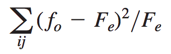
where f₀ represents observed frequencies in each cell of the table and F_e represents the expected frequencies in each cell under the null hypothesis of independence (no association) between the two variables. Summation is over all cells in the two- way table. If the goodness-of-fit tests for the two marginal effects are also computed, the usual χ² tests for the 2 one- way and 1 two-way effects do not sum to total x2 . This situation is similar to that of unequal-n ANOVA, where F tests of main effects and interactions are not independent. Because overlapping variance cannot be unambiguously assigned to effects, and because overlapping variance is repeatedly analyzed, interpretation of results is not clear- cut. In multiway frequency tables, as in ANOVA, nonadditivity of χ² becomes more serious as additional variables produce higher order (e.g., three-way and four-way) associations.

How do you calculate the likelihood ratio statistic?

An alternative strategy is to use the likelihood ratio statistic, G². The likelihood ratio statistic is distributed as χ² so the χ² tables can be used to evaluate significance. However, under certain conditions, G² has the property of additivity of effects. For example, in a twoway analysis:

G²_T = G²_A + G²_B + G²_AB 

The test of overall association within a two- way table, G²_T is the sum of the first- order goodness-of-fit tests, G²_A and G²_B and the G²_AB test of association, G², like χ², has a single equation for its various manifestations that differ among themselves only in how the expected frequencies are found.

G² = 2 Σ(f₀)ln(f₀>F_e)  

For each cell, the natural logarithm of the ratio of obtained to expected frequency is multiplied by the obtained frequency. These values are summed over cells, and the sum is doubled to produce the likelihood ratio statistics.

How do you screen for effects?

Screening is done if the researcher is data snooping and wishes simply to identify statistically significant effects. Screening is also done if the researcher hypothesizes a full model, a model with all possible effects included. Screening is not done if the researcher has hypothesized an incomplete model, a model with some effects included and others eliminated; in this case, the hypothesized model is tested and evaluated, followed by, perhaps, post hoc analysis.

The first step in screening is to determine if there are any effects to investigate. If there are, then screening progresses to a computation of Fe for each effect, a test of the reliability (significance) of each effect (finding G² for the first-order effects, the second-order or two-way associations, the third- order or three- way associations, and so on), and an estimation of the size of the statistically significant effects. Because the latter equation is used for all tests of the observed frequencies (f₀), the trick is to find the Fe necessary to test the various hypotheses.

How do you calculate an effect?

If done by hand, the process starts by calculation of overall G²_T which is used to test the hypothesis of no effects in the table (the hypothesis that all cells have equal frequencies). If this hypothesis cannot be rejected, there is no point to proceeding further. (Note that when all effects are tested simultaneously, as in computer programs, one can test either G²_T or G² for each of the effects, but not both, because degrees of freedom limit the number of hypotheses to be tested.) For the test of total effect:

F_e = N/rsp

Expected frequencies, F_e, for testing the hypothesis of no effects are the same for each cell in the table and are found by dividing the total frequency (N) by the number of cells in the table.

What does modelling entail?

In some applications of multiway frequency analysis, results of screening provide sufficient information for the researcher. In the current example, for instance, the results are clear- cut. One first- order effect, preference for reading type, is statistically significant, as is the sex-by-profession association. Often, however, the results are not so evident and consistent, and/or the goal is to find the best model for predicting frequencies in each cell of the design. A log- linear model is developed where an additive regression- type equation is written for (the log of) expected frequency as a function of the effects in the design. The procedure is similar to multiple regression, where a predicted DV is obtained by combining the effects of several IVs. A full model includes all possible effects in a multiway frequency analysis. The full model for a three-way design of the example is:

ln F_eijk = θ + λ_Ai + λBj + λCk + λABij+ λACik + λBCjk + λABCijk

For each cell (the natural logarithm of), the expected frequency, ln F_e, is an additive sum of the effect parameters, ls, and a constant, θ. For each effect in the design, there are as many values of λ - called effect parameters - as there are levels in the effect, and these values sum to zero. 

The purpose of modeling is to find the incomplete model with the fewest effects that still closely mimics the observed frequencies. Screening is done to avoid the necessity of exploring all possible incomplete models, an inhumane effort with large designs, even with computers. Effects that are found to be nonsignificant during the screening process are often omitted during modelling.

What different types of modelling do we distinguish?

Models come in two flavors, hierarchical and nonhierarchical.

• Hierarchical (nested) models include the highest- order statistically significant association and all its component parts.
• Nonhierarchical models do not necessarily include all the components. 

For hierarchical models, the optimal model is one that is not significantly worse than the next most complex one. Therefore, the choice among hierarchical models is made with reference to statistical criteria. There are no statistical criteria for choosing among nonhierarchical models and they are not recommended.

How do evaluation and interpretation work?

The optimal model, once chosen, is evaluated in terms of both the degree of fit to the overall data matrix (as discussed in the previous section) and the amount of deviation from fit in each cell.

Once a model is chosen, expected frequencies are computed for each cell and the deviation between the expected and the observed frequencies in each cell (the residual) is used to assess the adequacy of the model for fitting the observed frequency in that cell. In some cases, a model predicts the frequencies in some cells well, and in others very poorly, to give an indication of the combination of levels of variables for which the model is and is not adequate. Rather than trying to interpret raw differences, residuals usually are standardized by dividing the difference between observed and expected frequencies by the square root of the expected frequency to produce a z value. 

How do you calculate parameter estimates?

There is a different linear combination of parameters for most cells, and the sizes of the parameters in a cell reflect the contribution of each of the effects in the model to the frequency found in that cell. Parameters are estimated for the model from the F_e in a manner that closely follows ANOVA. In ANOVA, the size of an effect for a cell is expressed as a deviation from the grand mean. Each cell has a different combination of deviations that correspond to the particular combination of levels of the statistically significant effects for that cell. In MFA, deviations are derived from natural logarithms of proportions: ln (P_ijk). Expected frequencies for the model are converted to proportions by dividing F_e for each cell by N and then the proportions are changed to natural logarithms. 

• The first step is to find both the overall mean and the mean (in natural logarithm units) for each level of each of the effects in the model. In the first step, various means are found by summing ln (Pijk) across appropriate cells and dividing each sum by the number of cells involved.
• The second step is to express each level of each effect as a deviation from the overall mean. In the second step, parameter estimates are found by subtraction. For first-order effects, the overall mean is subtracted from the mean for each level.
• The third step is to convert the deviations to standard scores to compare the relative contributions of various parameters to the frequency in a cell.

What are the important differences between hierarchical and nonhierarchical models?

A model is hierarchical, or nested, if it includes all the lower effects contained in the highest-order association that is retained in the model. A hierarchical model for a four-way design, ABCD, with a significant three-way association, ABC, is A*B*C, A*B, A*C, B*C, and A, B, and C. The hierarchical model might or might not also include some of the other two-way associations and the D first-order effect.

A nonhierarchical model derived from the same four-way design includes only the significant two-way associations and first-order effects along with the significant threeway association; that is, a nonsignificant B*C association is included in a hierarchical model that retains the ABC effect but is not included automatically in a nonhierarchical model.

In log-linear analysis of multiway frequency tables, hierarchical models are the norm. Nonhierarchical models are suspect because higher order effects are confounded with lower order components. Therefore, it is best to explicitly include component lower order associations when specifying models in general log-linear programs. One major advantage of hierarchical models is the availability of a significance test for the difference between models, so that the most parsimonious adequately fitting model can be identified using inferential procedures. With nonhierarchical models, a statistical test for the difference between models is not available unless one of the candidate models happens to be nested in the other. IBM SPSS LOGLINEAR and GENLOG, and SAS CATMOD have the Newton–Raphson algorithm for assessing models and are considered general log- linear programs because they do not automatically impose hierarchical modeling. IBM SPSS HILOGLINEAR is restricted to hierarchical models.

What are the statistical criteria in multiway frequency analysis?

A potential source of confusion is that tests of models look for statistical nonsignificance while tests of effects look for statistical significance. Both kinds of tests commonly use the same statistics - forms of χ².

• When testing models, both Pearson χ² and the likelihood ratio statistic G² are often available for screening for the complexity of model necessary to fit data and for testing overall fit of models. Between the two, consistency favors use of G² because it is available for testing overall fit, screening, and testing for differences among hierarchical models. Also, under some conditions, inadequate expected frequencies can inflate Type I error rate when Pearson χ² is used.
• When testing individual effects, Two types of tests typically are available for testing individual effects in multiway frequency tables: chi- square tests of partial effects and z tests for single df parameter estimates. IBM SPSS HILOGLINEAR and SAS CATMOD provide partial G² tests of all effects in a full model. In addition, all programs print parameter estimates and their standard errors, which are converted to z tests of parameters or, in the case of SAS, χ² tests. However, IBM SPSS HILOGLINEAR prints these only for saturated models. IBM SPSS LOGLINEAR and GENLOG provide parameter estimates and their associated z tests, but no omnibus test for any effect that has more than one degree of freedom. If an effect has more than two levels, there is no single inferential test of that effect.

What is the strategy for choosing a model?

If you have one or more models hypothesized a priori, then there is no need for the strategies discussed in this section. The techniques in this section are used if you are building a model, or trying to find the most parsimonious incomplete model. As in all exploratory modeling, care should be taken in overgeneralizing results which may be subject to overfitting and inflated Type I error. Strategies for choosing a model differ depending on whether you are using IBM SPSS or SAS. Options and features differ among programs. You may find it handy to use one program to screen and another to evaluate models. Recall that hierarchical programs automatically include lower order components of higher order associations; general log- linear programs require that you explicitly include lower order components when specifying candidate hierarchical models.

• The IBM SPSS HILOGLINEAR Hierarchical program provides a test of each individual effect (with partial χ² reported where appropriate), simultaneous tests of all k-way effects (all one- way effects combined, all twoway effects combined, and so on), and simultaneous tests of all k-way and higher way effects (with a four-way model, all three-way and four-way effects combined, all two-way, three-way, and four way effects combined, and so on). Both Pearson and likelihood ratio χ² (G²) are reported. 
• The IBM SPSS GENLOG (general log-linear) program provides neither simultaneous tests for associations nor a stepping algorithm. Therefore, the procedure for choosing an appropriate model is simpler but less flexible.
• Finally, the SAS CATMOD and IBM SPSS LOGLINEAR (general log-linear) programs have no provision for stepwise model building and no simultaneous tests of association for each order. However, they do provide separate tests for each effect in a model, including effects with more than 1 df. A preliminary run with a full model, then, is used to identify candidates for model testing through the maximum likelihood chi-square test of association. 

How can you use SPSS for handling multiway frequency tables?

Currently there are two programs for handling multiway frequency tables in the package: HILOGLINEAR, which deals with only hierarchical models, and GENLOG, which deals with hierarchical and nonhierarchical models.

• IBM SPSS HILOGLINEAR, labeled Model Selection in the Loglinear menu, is well suited to choosing among hierarchical models, with several options for controlling stepwise selection of effects. Simultaneous tests of all k-way effects and of all k-way and higher effects are available for a quick screening of the complexity of the model from which to start stepwise selection. Parameter estimates and partial tests of association are available, but only for full models.
• IBM SPSS GENLOG does not provide stepwise selection of hierarchical models, although it can be used to compare user specified models of any sort. The program permits specification of continuous covariates. Also available is a simple specification of a logit model (in which one factor is a DV). Specification of a cell weighting variable must occur outside the GENLOG program.

No inferential tests of model components are provided in the program. Parameter estimates and their z tests are available for any specified model, along with their 95% confidence intervals. However, the parameter estimates are reported by single degrees of freedom, so that a factor with more than two categories has no omnibus significance test reported for either its main effect or its association with other effects. No quick screening for k-way tests is available. Screening information can be gleaned from a full model run, but identifying an appropriate model may be tedious with a large number of factors. Both IBM SPSS programs offer residuals plots. IBM SPSS GENLOG is the only program offering specification of Poisson models, which do not require that the analysis be conditional on total sample size.

How can you use SAS system for handling multiway frequency tables?

SAS CATMOD is a general program for modeling discrete data, of which log- linear modeling is only one type. The program is primarily set up for logit analyses where one variable is the DV but provision is made for log- linear models where no such distinction is made. The program offers simple designation of logit models, contrasts, and single df tests of parameters as well as maximum likelihood tests of more complex components. The program lacks provision for continuous covariates and stepwise model building procedures. SAS CATMOD uses different algorithms from the other three programs both for parameter estimation and model testing. 

How can you use SYSTAT system for handling multiway frequency tables?

SYSTAT LOGLIN is a general program for log- linear analysis of categorical data. The program uses its typical MODEL statement to set up the full, saturated, model (i.e., observed frequencies) on the left- hand side of the equation, and the desired model to be tested on the right- hand side. Structural zeros can be specified, and several options are available for controlling the iterative processing of model estimation. All of the usual descriptive and parameter estimate statistics are available, as well as multiple tests of effects in the model, both hierarchical and nonhierarchical. The program also prints outlying cells, designated 'outlandish'. Estimated frequencies and parameter estimates can be saved to a file.

In summary, what does the General Linear Model look like? - Chapter 17

How does linearity relate to the general linear model?

To facilitate choice of the most useful technique to answer your research question, the emphasis has been on differences among statistical methods. We have repeatedly hinted, however, that most of these techniques are special applications of the general linear model (GLM). The goal of this chapter is to introduce the GLM and to fit the various techniques into the model. In addition to the aesthetic pleasure provided by insight into the GLM, an understanding of it provides a great deal of flexibility in data analysis by promoting use of more sophisticated statistical techniques and computer programs. Most data sets are fruitfully analyzed by one or more of several techniques.

Linearity and additivity are important to the GLM. Pairs of variables are assumed to have a linear relationship with each other; that is, it is assumed that relationships between pairs of variables are adequately represented by a straight line. Additivity is also relevant, because if one set of variables is to be predicted by a set of other variables, the effects of the variables within the set are additive in the prediction equation. The second variable in the set adds predictability to the first one, the third adds to the first two, and so on. In all multivariate solutions, the equation relating sets of variables is composed of a series of weighted terms added together. These assumptions, however, do not prevent inclusion of variables with curvilinear or multiplicative relationships. As discussed throughout this book, variables can be multiplied together, raised to powers, dichotomized, transformed, or recoded so that even complex relationships are evaluated within the GLM.

What does the bivariate form look like?

The GLM is based on prediction or, in jargon, regression. A regression equation represents the value of a DV, Y, as a combination of one or more IVs, Xs, plus error. The simplest case of the GLM, then, is the familiar bivariate regression:

A + BX + e = Y

where, B is the change in Y associated with a one-unit change in X; A is a constant representing the value of Y when X is 0; and e is a random variable representing error of prediction.

If X and Y are converted to standard z-scores, z_x and z_y, they are now measured on the same scale and cross at the point where both z-scores equal 0. The constant A automatically becomes 0 because z_y is 0 when z_x is 0. Further, after standardization of variances to 1, slope is measured in equal units (rather than the possibly unequal units of X and Y raw scores) and now represents the strength of the relationship between X and Y; in bivariate regression with standardized variables, it is equal to the Pearson product- moment correlation coefficient. The closer β is to 1.00 or -1.00, the better the prediction of Y from X (or X from Y). The equation then simplifies to:

βz_x + e = zy

What is one important distinction in statistics?

One distinction that is sometimes important in statistics is whether data are continuous or discrete. There are, then, three forms of bivariate regression for situations where X and Y are (1) both continuous - analyzed by Pearson product-moment correlation, (2) mixed, with X dichotomous and Y continuous - analyzed by point biserial correlation, and (3) both dichotomous - analyzed by phi coefficient. In fact, these three forms of correlation are identical. If the dichotomous variable is coded 0– 1, all the correlations can be calculated using the equation for Pearson product- moment correlation.

What does the simple multivariate form look like?

The first generalization of the simple bivariate form of the GLM is to increase the number of IVs, Xs, used to predict Y. It is here that the additivity of the model first becomes apparent. In standardized form:

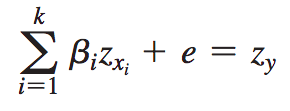
That is, Y is predicted by a weighted sum of Xs. The weights, bi, no longer reflect the correlation between Y and each X because they are also affected by correlations among the Xs. Here again there are special statistical techniques associated with whether all Xs are continuous; here also, with appropriate coding, the most general form of the equation can be used to solve all the special cases. If Y and all Xs are continuous, the special statistical technique is multiple regression.

The latter equation is used to describe the multiple regression problem. But if Y is continuous and all Xs are discrete, we have the special case of regression known as analysis of variance. The values of X represent 'groups' and the emphasis is on finding mean differences in Y among groups rather than on predicting Y, but the basic equation is the same. A significant difference among groups implies that knowledge of X can be used to predict performance on Y.

How can analysis of variance problems be solved?

Analysis of variance problems can be solved through multiple regression computer programs. There are as many Xs as there are degrees of freedom for the effects. For example, in a one way design, three groups are recoded into two dichotomous Xs - one representing the first group versus the other two and the second representing the second group versus the other two. The third group is those who are not in either of the other two groups. Inclusion of a third X would produce singularity because it is perfectly predictable from the combination of the other two.

• If IVs are factorially combined, main effects and interactions are still coded into a series of dichotomous X variables.
• If some Xs are continuous and others are discrete, with Y continuous, we have analysis of covariance. The continuous Xs are the covariates and the discrete ones are the IVs. The effects of IVs on Y are assessed after adjustments are made for the effects of the covariates on Y. Actually, the GLM can deal with combinations of continuous and discrete Xs in much more general ways than traditional analysis of covariance, as alluded to in Chapters 5 and 6.
• If Y is dichotomous (two groups), with Xs continuous, we have the simple multivariate form of discriminant analysis. The aim is to predict group membership on the basis of the Xs. There is a reversal in terminology between ANOVA and discriminant analysis; in ANOVA the groups are represented by X, but in discriminant analysis the groups are represented by Y. The distinction, although confusing, is trivial within the GLM. As seen in forthcoming sections, all the special techniques are simply special cases of the full GLM.
• If Y and all Xs are discrete, we have multiway frequency analysis. The log-linear model, rather than the simple linear model, is required to evaluate relationships among variables. Logarithmic transforms are applied to cell frequencies and the weighted sum of these cell frequencies is used to predict group membership. Because the equation eventually boils down to a weighted sum of terms, it is considered here to be part of the GLM.
• If Y is dichotomous and Xs are continuous and/or discrete, we have logistic regression analysis. Again a nonlinear model, in this case the logistic model, is required to evaluate relationships among variables. Y is expressed in terms of the probability of being in one or the other level. The linear regression equation is the (natural log of the) probability of being in one group divided by the probability of being in the other group. Because the linear regression equation does appear in the model, it can be considered part of the GLM.
• Multilevel modeling deals with a hierarchy of Ys and Xs and equations to relate them. At the first level, Ys may be individual scores for each case on a single DV, individual scores for each case at a particular time (repeated- measures application of MLM) on a single DV, or scores for each case on multiple DVs. Ys at subsequent levels are intercepts and/or slopes over units at lower levels. Xs at each level are predictors of scores at that level. Although there are multiple Ys at each level except the first one (and even at the first one if there is more than one DV) and may be multiple Xs, they are never formed into combinations. Therefore, this is not a true multivariate strategy.
• If Y is continuous and is the time it takes for something to happen, we have survival analysis. Xs can be continuous covariates and/or treatment(s), dichotomously coded. Here the equation is based on a log- linear rather than a linear model, but like logistic regression may be considered part of the GLM. The difference between logistic regression and survival analysis is that the Y in logistic regression is the probability of something happening and in survival analysis the Y is how long it takes to happen.
• In time-series analysis, Y is continuous, and one X is always time. Intervention studies also require at least one dichotomous X, usually a treatment but rarely experimentally manipulated.

What does the full multivariate form look like?

The GLM takes a major leap when the Y side of the equation is expanded because more than one equation may be required to relate the Xs to the Ys:

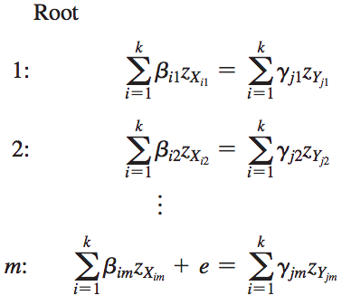
where m equals k or p, whichever is smaller, and γ are regression weights for the standardized Y variables.

In general, there are as many equations as the number of X or Y variables, whichever is smaller. When there is only one Y, Xs are combined to produce one straight- line relationship with Y. Once there is more than one Y, however, combined Ys and combined Xs may fit together in several different ways. Each combination of Ys and Xs is a root. Roots are called by other names in the special statistical technique in which they are developed: discriminant functions, principal components, canonical variates, and so forth. Full multivariate techniques need multidimensional space to describe relationships among variables. With 2 df, two dimensions might be needed. With 3 df, up to three dimensions might be needed, and so on.

The number of roots necessary to describe the relationship between two sets of variables may be smaller than the number of roots maximally available. For this reason, the error term for Equation 17.4 is not necessarily associated with the mth root. It is associated with the last necessary root, with “necessary” statistically or psychometrically defined.

What analyses can you conduct in different cases of continuous or non-continuous variables?

As with simpler forms of the GLM, specialized statistical techniques are associated with whether variables are continuous.

• Canonical correlation is the most general form and the noble ancestor of the GLM where all Xs and Ys are continuous. 
• With all Xs discrete and all Ys continuous, we have multivariate analysis of variance. The discrete X variables represent groups, and combinations of Y variables are examined to see how their centroids differ as a function of group membership. If some Xs are continuous, they can be analyzed as covariates, just as in ANCOVA; MANCOVA is used to discover how groups differ on Ys after adjustment for the effects of covariates.
• If the Ys are all measured on the same scale and/or represent levels of a within- subjects IV, profile analysis is available - a form of MANOVA that is especially informative for these kinds of data. And if there are multiple DVs at each level of a within-subjects IV, doubly multivariate analysis of variance is used to discover the effects of the IVs on the Ys.
• When Y is discrete (more than two groups) and Xs are continuous, the full multivariate form of discriminant analysis is used to predict membership in Y.
• In structural equations modeling, continuous and latent variables are acceptable on both sides of the equations—the X side as well as the Y side. For each Y, whether continuous (an observed indicator variable) or latent (a factor composed of multiple observed indicator variables), there is an equation involving continuous and/or latent Xs. Ys for some equations may serve as Xs for other equations, and vice versa. It is these equations that render structural equations modeling part of the GLM.
• Finally, if Y is discrete and Xs are continuous and/or discrete, we have logistic regression analysis. As for MFA, a nonlinear model, the logistic model, is required to evaluate relationships among variables. Y is expressed in terms of the probability of being in one versus any of the other levels, with a separate equation for each level of Y but one. For each equation, the linear regression equation is the (natural log of the) probability of being in one group divided by the probability of being in any of the other groups. Because the model includes the linear regression equation, it can be considered part of the GLM.

What alternative research strategies are there?

For most data sets, there is more than one appropriate analytical strategy, and choice among them depends on considerations such as how the variables are interrelated, your preference for interpreting statistics associated with certain techniques, and the audience you intend to address.

A data set for which alternative strategies are appropriate has groups of people who receive one of three types of treatments: behavior modification, short- term psychotherapy, or a waiting- list control group. Suppose a great many variables are measured— self- reports of symptoms and moods, reports of family members, therapist reports, and a host of personality and attitudinal tests - the major goal of the analysis is probably to find out if, and on which variable(s), the groups differ after treatment. The obvious strategy is MANOVA, but a likely problem is that the number of variables exceeds the number of clients in some group, leading to singularity. Further, with so many variables, some are likely to be highly related to combinations of others. You could choose among them or combine them on some rational basis, or you might choose first to look at empirical relationships among them. 

• A first step in reducing the number of variables might be examination of squared multiple correlations of each variable with all the others through regression or factor analysis programs. But the SMCs might or might not provide sufficient information for a judicious decision about which variables to delete and/or combine. If not, the next likely step is a principal component analysis on the pooled within- cells correlation matrix.
• The usual procedures for deciding the number of components and type of rotation are followed. Out of this analysis come scores for each client on each component and some idea of the meaning of each component. Depending on the outcome, subsequent strategies might differ. If the principal components are orthogonal, the component scores can serve as DVs in a series of univariate ANOVAs, with adjustment for experimentwise Type I error. If the components are correlated, then MANOVA is used with component scores as DVs. The stepdown sequence might well correspond to the order of components (the scores on the first component enter first, and so on).
• Or you might want to analyze the component scores through a discriminant analysis to learn, for instance, that differences between behavior modification and short- term psychotherapy are most notable on components loaded heavily with attitudes and self- reports, but differences between the treated groups and the control group are associated with components loaded with therapist reports and personality measures.
• You could, in fact, solve the entire problem through discriminant analysis or logistic regression. Both types of analyses protect against multicollinearity and singularity by setting a tolerance level so that the variables that are highly predicted by the other variables do not participate in the solution. Logistic regression is especially handy when the predictors are a mix of many different types of variables. 

What does time-series analysis entail? - Chapter 18

What is the general purpose of time-series analysis?

Time-series analysis is used when observations are made repeatedly over 50 or more time periods. Sometimes, the observations are from a single case, but more often they are aggregate scores from many cases. One goal of the analysis is to identify patterns in the sequence of numbers over time, which are correlated with themselves, but offset in time. Another goal in many research applications is to test the impact of one or more interventions (IVs). Time-series analysis is also used to forecast future patterns of events or to compare series of different kinds of events.

As in other regression analyses, a score is decomposed into several potential elements. One of the elements is a random process, called a shock. Shocks are similar to the error terms in other analyses. Overlaying this random element are numerous potential patterns.

• One potential pattern is trends over time is the linear pattern. Here, the mean is steadily increasing or decreasing over time. Also, there is the quadratic pattern, where the mean first increases and then decreases over time, or the reverse. 
• Another potential pattern is lingering effects of earlier scores.
• The third potential pattern is lingering effects of earlier shocks. These patterns are not mutually exclusive; two or all three can be superimposed on the random process.

What is the auto-regressive model?

The model described in this chapter is the auto-regressive, integrated, moving average, called an ARIMA (p, d, q) model.

• The auto-regressive element, p, represents the lingering effects of the preceding scores.
• The integrated element, d, represents trends in the data.
• The moving average element, q, represents the lingering effects of preceding random shocks.

What are the steps of time-series analysis?

The first three steps in the analysis are identification, estimation, and diagnosis. These steps are devoted to modelling the patterns in the data.

1. The first step is identification, in which autocorrelation functions (ACFs) and partial autocorrelation functions (PACFs) are examined to see which of the potential three patterns are present in the data. Autocorrelations are self-correlations of the series of scores with itself, removed one or more periods in time; partial autocorrelations are self-correlations with intermediate autocorrelations partialed out. Various auto-regressive and moving average patterns leave distinctive footprints on the autocorrelation and partial autocorrelation functions.
2. The second step in modeling the series is estimation in which the estimated size of a lingering auto-regressive or moving average effect is tested against the null hypothesis that it is zero. 
3. The third step is diagnosis, in which residual scores are examined to determine if there are still patterns in the data that are not accounted for. Residual scores are the differences between the scores predicted by the model and the actual scores for the series. If all patterns are accounted for in the model, the residuals are random. In many applications of time series, identifying and modelling the patterns in the data are sufficient to produce an equation, which is then used to predict the future of the process. This is called forecasting, the goal of many applications of time series in the economic arena.

What is the goal of time-series analysis?

However, often the goal is to assess the impact of an intervention. The intervention is occasionally experimental, featuring random assignment of cases to the levels of treatment, control of other variables, and manipulation of the levels of the IV by the researcher.

An intervention is tested for significance in the traditional manner, once the endogenous patterns in the data have been reduced to error through modeling. The effects of interventions considered in this chapter vary in both onset and duration; the onset of the effect may be abrupt or gradual and the duration of the effect may be either permanent or temporary. Effects of interventions are superimposed on the other patterns in the data. 

In what situation is a repeated measures ANOVA more appropriate?

True experiments typically assess the DV far fewer than 50 times and therefore cannot use time-series analysis. More likely with experiments, there is a single measure before the intervention (a pretest) and, perhaps, a few measures after the intervention to assess immediate and follow-up effects. In this situation, repeated measures ANOVA is more appropriate as long as heterogeneity of covariance (sphericity) is taken into account.

What kinds of research questions can be tested with time-series analysis?

The major research questions involve the patterns in the series, the predicted value of the scores in the near future, and the effect of an intervention (an IV). Less common questions address the relationships among time series. It should be understood that this chapter barely scratches the surface of the complex world of time-series analysis. Only those questions that are relatively easily addressed in IBM SPSS and SAS are discussed.

• The first type of research questions it can be used for is patterns of autocorrelation. The pattern of autocorrelation is modelled in any time-series study, for itself, in preparation for forecasting, or prior to tests of an intervention. Are there linear or quadratic trends in the data? Does the previous score affect the current one or the previous random shock? How quickly do autocorrelations die out over time?
• Another type of research questions relate to seasonal cycles and trends. Time-series data are also examined for seasonal cycles if such are possible. Are there weekly, quarterly, monthly, or yearly trends in the data?
• The third type of research questions time-series analysis can be used for is for forecasting. Based on the known patterns in the data, what is the predicted value of observations in the near future?
• Then, time-series analysis can also be used to test the effect on an intervention. Has an intervention had an impact, after taking into account patterns in the scores associated with trends, auto-regression, moving averages, and periodicity? Intervention is added to a model as an IV. 
• Furthermore, it can be used to compare time series. Are the patterns over time similar for different variables or populations?
• Then, it can also be used for time series with covariates. Covariates, often called predictors in time-series jargon, may be measured along with the DV. A first question is, is the covariate related to the DV, after adjusting both for autocorrelation and periodicity?
• Effect size and power can also be tested for. How much of the variability in observations is due to the chosen model? Power depends on the accuracy of ARIMA modelling, as well as on the number of observations over time and the impact of the intervention.

What are the theoretical assumptions of time-series analysis?

The usual cautions apply with regard to causal inference in time-series analysis. Only with random assignment to treatment conditions, control of extraneous variables, and manipulation of the intervention(s) can cause reasonably be inferred when differences associated with an intervention are observed. Quasi-experiments are designed to rule out as many alternative sources of influence on the DV as possible, but causal inference is much weaker in any design that falls short of the requirements of a true experiment.

What are some practical issues of time-series analysis?

The random shocks that perturb the system are considered to be independent and normally distributed with mean zero and constant variance over time. Contingencies among scores over time are part of the model that is developed during identification and estimation. If the model is good, all sequential contingencies are removed so that you are left with the randomly distributed shocks. The residuals, then, are a reflection of the random shocks: independent and normally distributed, with mean zero and homogeneity of variance. It is expressly assumed that there are correlations in the sequence of observations over time that have been adequately modeled. This assumption is tested during the diagnostic phase when remaining, as yet unaccounted for patterns are sought among the residuals. Outliers among scores are sought before modelling and among the residuals once the model is developed.

What are the four assumptions of time-series analysis?

Time-series analysis has four assumptions that need to be met:

• A model is developed and then normality of residuals is evaluated in time-series analysis. Examine the normalized plot of residuals for the model before evaluating an intervention. Transform the DV if residuals are nonnormal. The normalized plot of residuals is examined as part of the diagnostic phase of modelling.
• After the model is developed, examine plots of standardized residuals versus predicted values to assess homogeneity of variance over time. Consider transforming the DV if the width of the plot varies over the predicted values.
• Time series data inherently violate the assumption of independence of residuals because of autocorrelations over time; indeed, the purpose of the identification process is to identify and deal with these dependencies. During the diagnostic phase, once the model is developed and residuals are computed, there should be no remaining autocorrelations or partial autocorrelations at various lags in the ACFs and PACFs. Remaining autocorrelations at various lags signal other possible patterns in the data that have not been properly modeled. Examine the ACFs and PACFs for other patterns and adjust the model accordingly..
• Outliers are observations that are highly inconsistent with the remainder of the time-series data. They can greatly affect the results of the analysis and must be dealt with. They sometimes show up in the original plot of the DV against time, but are often more noticeable after initial modeling is complete. Examine the time-series plot before and after adjusting for autocorrelation and seasonality to identify obvious outliers.

What are the fundamental equations used in time-series ARIMA models?

The ARIMA (auto-regressive, integrated, moving average) model of a time series is defined by three terms (p, d, q). Identification of a time series is the process of finding integer, usually very small (e.g., 0, 1, or 2), values of p, d, and q that model the patterns in the data. When the value is 0, the element is not needed in the model. The middle element, d, is investigated before p and q. The goal is to determine if the process is stationary and, if not, to make it stationary before determining the values of p and q. Recall that a stationary process has a constant mean and variance over the time period of the study.

What is the first step in time-series analysis?

The first step in the analysis is to plot the sequence of scores over weeks by selecting Graphs, and then Sequence. The two relevant features of the plot are central tendency and dispersion. Is the mean apparently shifting over the time period? Is the dispersion increasing or decreasing over the time period?

There are possible shifts in both the mean and the dispersion over time for this series. The mean may be edging upwards, and the variability may be increasing. If the mean is changing, the trend is removed by differencing once or twice. If the variability is changing, the process may be made stationary by logarithmic transformation. Differencing the scores is the easiest way to make a nonstationary mean stationary (flat). The number of times you have to difference the scores to make the process stationary determines the value of d. If d = 0, the model is already stationary and has no trend. When the series is differenced once, d = 1 and linear trend is removed. When the difference is then differenced, d = 2 and both linear and quadratic trend are removed. For nonstationary series, d values of 1 or 2 are usually adequate to make the mean stationary. Differencing simply means subtracting the value of an earlier observation from the value of a later observation. 

How do you calculate the random shock at a specific time period?

In the simplest time series, an observation at a time period simply reflects the random shock at that time period, at, that is:

Y_t = ai

The random shocks are independent, with constant mean and variance, and so are the observations. If there is trend in the data, however, the score also reflects that trend as represented by the slope of the process. In this slightly more complex model, the observation at the current time, Yt, depends on the value of the previous observation, Yt-1 the slope, and the random shock at the current time period:

Y_t = θ₀(Y_t-1)+at

To see if the process is stationary after linear trend is removed, the first difference scores at lag 1 are plotted against weeks. If the process is now stationary, the line will be basically horizontal with constant variance.The series now appears stationary with respect to central tendency, so second differencing does not appear necessary. However, the variability seems to be increasing over time. Transformation is considered for series in which variance changes over time and differencing does not stabilize the variance.

How do you calculate the auto-regressive components?

The auto-regressive components represent the memory of the process for preceding observations. The value of p is the number of auto-regressive components in an ARIMA (p, d, q ) model. The value of p is 0 if there is no relationship between adjacent observations. When the value of p is 1, there is a relationship between observations at lag 1 and the correlation coefficient φ₁ is the magnitude of the relationship. When the value of p is 2, there is a relationship between observations at lag 2 and the correlation coefficient φ₂ is the magnitude of the relationship. Thus, p is the number of correlations you need to model the relationship. For example, a model with p = 2, ARIMA (2, 0, 0), is:

Y_t = ϕ₁Yt-1 + ϕ₂Y_t-2 + a_t

How do you calculate a moving average component?

The moving average components represent the memory of the process for preceding random shocks. The value q indicates the number of moving average components in an ARIMA (p, d, q ) model. When q is zero, there are no moving average components. When q is 1, there is a relationship between the current score and the random shock at lag 1, and the correlation coefficient u1 represents the magnitude of the relationship. When q is 2, there is a relationship between the current score and the random shock at lag 2, and the correlation coefficient u2 represents the magnitude of the relationship. Thus, an ARIMA (0, 0, 2) model is:

Y_t = at - θ₁a_t-1 - θ₂a_t-2

What is the formula in the case of mixed models?

Somewhat rarely, a series has both auto-regressive and moving average components so both types of correlations are required to model the patterns. If both elements are present only at lag 1, the equation is:

Y_t = ϕ₁Y_t-1 - θ₁a_t-1 + a_t

How can you calculate ACFs and PACFs?

Models are identified through patterns in their ACFs (autocorrelation functions) and PACFs (partial autocorrelation functions). Both autocorrelations and partial autocorrelations are computed for sequential lags in the series. The first lag has an autocorrelation between Y_t-1 and Y_t, the second lag has both an autocorrelation and partial autocorrelation between Y_t-2 and Y_t, and so on. ACFs and PACFs are the functions across all the lags. The equation for autocorrelation is similar to bivariate r except that the overall mean Y is subtracted from each Y_t and from each Y_t-k, and the denominator is the variance of the whole series.

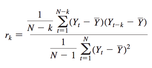
where N is the number of observations in the whole series and k is the lag. Y is the mean of the whole series and the denominator is the variance of the whole series.

The standard error of an autocorrelation is based on the squared autocorrelations from all previous lags. At lag 1, there are no previous autocorrelations, so r 2 0 is set to 0.

What is the equation for a partial autocorrelation?

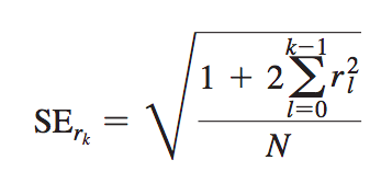
The equations for computing partial autocorrelations are much more complex, and involve a recursive technique. However, the standard error for a partial autocorrelation is simple and the same at all lags:

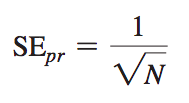
The series used to compute the autocorrelation is the series that is to be analyzed. Because differencing is used with the small-sample example to remove linear trend, it is the differenced scores that are analyzed. 

When is an autocorrelation included in the ARIMA model?

If an autocorrelation at some lag is significantly different from zero, the correlation is included in the ARIMA model. Similarly, if a partial autocorrelation at some lag is significantly different from zero, it is included in the ARIMA model as well. The significance of full and partial autocorrelations is assessed using their standard errors. Although you can look at the autocorrelations and partial autocorrelations numerically, it is standard practice to plot them. The center vertical (or horizontal) line for these plots represents full or partial autocorrelations of zero; then symbols such as * or _ or bars are used to represent the size and direction of the autocorrelation and partial autocorrelation at each lag. You compare these obtained plots with standard, and somewhat idealized, patterns that are shown by various ARIMA models.

The boundary lines around the functions are the 95% confidence bounds. The pattern here is a large, negative autocorrelation at lag 1 and a decaying PACF, suggestive of an ARIMA (0, 0, 1) model.

How can model parameters be estimated?

Estimating the values of parameters in models consists of estimating the f parameter(s) from an auto-regressive model or the parameter(s) from a moving average model. As indicated by McDowall and colleagues, the following rules apply:

• Parameters must differ significantly from zero and all significant parameters must be included in the model.
• Because they are correlations, all auto-regressive parameters, ϕ must be between -1 and 1. If there are two such parameters (p = 2) they must also meet the following requirements:

  ϕ₁ + ϕ₂ < 1 and ϕ₂ - ϕ₁ < 1

  These are called the bounds of stationarity for the auto-regressive parameter(s).

• Because they are also correlations, all moving average parameters, θ must be between -1 and 1. If there are two such parameters (q = 2), they must also meet the following requirements:

  θ₁ + θ₂ < 1 and θ₂ - θ₁ < 1 

  These are called the bounds of invertibility for the moving average parameter(s).

Complex and iterative maximum likelihood procedures are used to estimate these parameters. The reason for this is seen in an equation for θ₁ :

How can we diagnose a model?

How well does the model fit the data? Are the values of observations predicted from the model close to actual ones? If the model is good, the residuals (differences between actual and predicted values) of the model are a series of random errors. These residuals form a set of observations that are examined the same way as any time series. ACFs and PACFs for the residuals of the model are examined.

What are the different types of time-series analysis?

There are two major varieties of time-series analysis: time domain (including Box–Jenkins ARIMA analysis) and spectral domain (including Fourier spectral analysis).

• Time domain analyses deal directly with the DV over time;
• Spectral domain analyses decompose a time series into its sine wave components.

Either time or spectral domain analyses can be used for identification, estimation, and diagnosis of a time series. However, current statistical software offers no assistance for intervention analysis using spectral methods. As a result, this chapter is limited to time domain analyses. Numerous complexities are available with these analyses, however—seasonal autocorrelation and one or more interventions (and with different effects), to name a few.

When do you use a model with seasonal components?

Seasonal autocorrelation is distinguished from local autocorrelation in that it is predictably spaced in time. Observations gathered monthly, for example, are often expected to have a spike at lag 12 because many behaviors vary consistently from month to month over the year. Similarly, observations made daily could easily have a spike at lag 7, and observations gathered hourly often have a spike at lag 24. These seasonal cycles can often be postulated a priori, while local cycles are inferred from the data.

Like local cycles, seasonal cycles show up in plots of ACFs and PACFs as spikes. However, they show up at the appropriate lag for the cycle. Like local cycles, these autocorrelations can also be auto- regressive or moving average (or both). And, like local autocorrelation, a seasonal autoregressive component tends to produce a decaying ACF function and spikes on the PACF while a moving average component tends to produce the reverse pattern. When there are both local and seasonal trends, d, multiple differencing is used. Seasonal models may be either additive or multiplicative.

When do you use a model with interventions?

Intervention, or interrupted, time-series analyses compare observations before and after some identifiable event. In quasi- experiments, the intervention is an attempt at experimental manipulation; however, the techniques are applicable to analysis of any event that occurs during the time series. The goal is to evaluate the impact of the intervention. Interventions differ in both the onset (abrupt or gradual) and duration (permanent or temporary) of the effects they produce.

The connection between an intervention and its effects is called a transfer function. In time-series jargon, an impulse intervention is also called an impulse or a pulse indicator and the effect is called an impulse or a pulse function. An effect with abrupt onset and permanent or long duration is called a step function. Because there are two levels of duration (permanent and temporary) and two levels of onset (abrupt and gradual), there are four possible combinations of effects, but the gradual-onset, short-term effect occurs rarely and requires curve fitting. Intervention analysis requires a column for the indicator variable that flags the occurrence of the event. With an impulse indicator, a code of 1 is applied in the indicator column at the single specific time period of the intervention and a code of 0 to the remaining time periods. When the intervention is of long duration or the effect is expected to persist, the column for the indicator contains 0s during the baseline time period and 1s at the time of and after the intervention.

How do you calculate the level change:

Intervention analysis begins with identification, estimation, and diagnosis of the observations before intervention. The model, including the indicator variable, is then re-estimated for the entire series and the results diagnosed. The effect of the intervention is assessed by interpreting the coefficients for the indicator variable.

Transfer functions have two possible parameters. The first parameter, ω, is the magnitude of the asymptotic change in level after intervention. The second parameter, δ, reflects the onset of the change, the rate at which the post-intervention series approaches its asymptotic level. The ultimate change in level is:

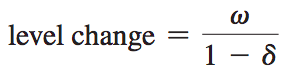
Both ω and δ are tested for significance. If the null hypothesis that ω is 0 is retained, there is no impact of intervention. If ω is significant, the size of the change is ω. The d coefficient varies between 0 and 1. When δ is 0 (nonsignificant), the onset of the impact is abrupt. When d is significant but small, the series reaches its asymptotic level quickly. The closer δ is to 1, the more gradual the onset of change. SAS permits specification and evaluation of both ω and δ but IBM SPSS permits evaluation only of ω.

What are abrupt, permanent effects?

Abrupt, permanent effects, called step functions, are those that are expected to show an immediate impact and continue over the long term. All post-intervention observations are coded 1 and ω is specified, but not δ (or it is specified as 0).

What are abrupt, temporary effects?

Now suppose that the intervention has a strong, abrupt initial impact that dies out quickly. This is called a pulse effect.

What are gradual, permanent effects?

Another possible effect of intervention is one that gradually reaches its peak effectiveness and then continues to be effective. The data set is the same as for an abrupt, permanent effect. However, now we are proposing that there is a linear growth in the effect of the intervention from the time it is implemented. 

Multiple interventions are modeled by specifying more than one IV. Several interventions can be included in models when using either IBM SPSS ARIMA or SAS ARIMA.

How do you add continuous variables?

Continuous variables are added to time-series analyses to serve several purposes.

• One is to compare time series over populations or over different conditions. 
• Another use is to add a continuous IV as a predictor. 
• Finally, one or more continuous IVs might be added as covariates to an intervention analysis.

These analyses have their own assumptions and limitations. As usual, use of a covariate assumes that it is not affected by the IV; for example, it is assumed that temperature is not affected by introduction of the profit-sharing plan in the company under investigation. 

What are some important issues with time-series analysis?

ARIMA models are identified by matching obtained patterns of ACF and PACF plots with idealized patterns. The best match often indicates which of the (p, d, q) parameters need to be included in the model, and at what size (0, 1, or 2). Sometimes, however, more than one pattern is suggested by the plots, or, like the small-sample example, the best pattern match does not reduce the residuals to random error. A first best guess is made on the basis of the ACF, PACF pattern and then, if the model fits the data poorly, another is tried out until the diagnostic phase is satisfactory.

• A “classic” auto-regressive model—ARIMA (p, 0, 0)—has an ACF that slowly approaches 0 and a PACF that spikes at lag p. Thus, if there is a spike only at lag 1 of the PACF (partial autocorrelation between Yt and Yt-1) and the ACF slowly declines, the model is probably ARIMA (1, 0, 0). If there is also a spike at lag 2 of the PACF (an autocorrelation between Yt and Yt-2 with Yt-1 partialed out) and the ACF slowly declines, the model is likely to be ARIMA (2, 0, 0). Thus, the number of spikes on the PACF indicates the value of p for auto-regressive models.
• A “classic” moving average model—ARIMA (0, 0, q)—has an ACF that spikes on the first q lags and a PACF that declines slowly. If there is a spike at lag 1 of the ACF and the PACF declines, the model may be ARIMA (0, 0, 1). If there also is a spike at lag 2 of the ACF and the PACF declines, the model is probably ARIMA (0, 0, 2). Thus, the number of spikes on the ACF indicates the value of q.
• A mixed auto-regressive, moving average model has a slowly declining ACF, from the autoregressive portion of the model (p), and also a slowly declining PACF, from the moving average portion of the model (q). The sizes of the auto-regressive and moving average parameters are not evident from the ACF and PACF. Therefore, it is prudent to start with p = 1 and q = 1 and increase these values only if residual ACF and PACF show spikes in the diagnostic phase. If the parameters are set too high, it may not show up in diagnosis, except perhaps as nonsignificant parameter estimates.
• A nonstationary model—ARIMA (0, 1, 0)—has a single PACF spike, but there are two common ACF patterns. There may be constant spikes or there may be a 'damped sine wave', in which spikes oscillate first on one side and then on the other side of zero autocorrelation.

If either an autocorrelation or a partial autocorrelation between observations k lags apart is statistically significant, the autocorrelation is included in the ARIMA model. The significance of an autocorrelation is evaluated from the 95% confidence intervals printed alongside it, or from the t distribution where the autocorrelation is divided by its standard error, or from the Box–Ljung statistic printed as standard IBM SPSS output. Alternatively, SAS ARIMA provides tests of sets of lags. 

How do you calculate effect sizes in time-series analysis?

Effect size in time- series analysis is based on evaluation of residuals after finding an acceptable model. If there is an intervention, the residuals after the intervention is modeled are compared with the residuals before the intervention is modeled.

Two measures of effect size are available.

• One is a goodness-of-fit statistic that is traditionally used with time-series analysis. The traditional goodness-of-fit measure for time-series analysis is the residual mean square. The residual mean square (RMS) is the average of the square root of the squared residual (ant ) values summed over the N time periods.

• The second, more interpretable, measure of effect size is R2 , which, as usual, reflects variance explained by the model as a proportion of total variance in the DV. The proportion of systematic variance explained by the model (R²) is one minus the sum of squared residuals divided by the sum of squared Y_t values, where Y_t is the difference-adjusted DV.

What does forecasting entail?

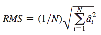
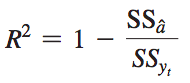
Forecasting refers to the process of predicting future observations from a known time series and is often the major goal in nonexperimental use of the analysis. However, prediction beyond the data is to be approached with caution. The farther the prediction beyond the actual data, the less reliable the prediction. And only a small percentage of the number of actual data points can be predicted before the forecast turns into a straight line.

What statistical methods can be used for comparing two models?

Often the identification process suggests two or more candidate models. Sometimes, however, both models fail to meet the criteria, or both meet all of the criteria. Statistical tests are available to determine whether two models are reliably different. The difference in AIC for the two models is evaluated as x² with df equal to the difference in the number of parameters for the two models.

x² (df) = AIC(smaller model) - AIC(larger model)

What statistical programs can be used for time-series analysis?

SAS and IBM SPSS each have a single program for ARIMA time-series modeling. IBM SPSS has additional programs for producing time-series graphs and for forecasting seasonally adjusted time series. SAS has a variety of programs for time-series analysis, including a special one for seasonally adjusted time series. SYSTAT also has a time-series program, but it does not support intervention analysis.

Source and more study assistance:

• Type: Book summary
• Book title: Using multivariate statistics
• Subtitle: Pearson New International Edition
• Author: Tabachnick
• Edition: 6th edition
• Study assistance: For all available summaries, practice questions, bulletpoints and examtips with the book, go to Study Guide for summaries with Using multivariate statistics: Pearson New International Edition by Tabachnick